L01 · Wildfire Percolation
Light one edge of a random forest. Does the fire make it to the other side? In a big forest, below a tree density of 59.27 % it almost never does. Above it, it almost always does. That one number, the percolation threshold $p_c$, is a doorway into phase transitions, scaling laws and self-organised criticality. All of it comes from a 4-neighbour grid rule you could explain to a ten-year-old.
You are here
Welcome to level 1 of 10. Each level jumps to a new field and adds tools to the stack. This one uses the smallest stack, just NumPy and Matplotlib, but the science is the real thing, and the habits you build here come back on every later level:
| Level | Field | M&S paradigm | New tools | |
|---|---|---|---|---|
| ▶ | L01 Wildfire Percolation | Statistical physics / ecology | Cellular automata, Monte Carlo, phase transitions | NumPy, Matplotlib |
| L02 Noise in Gene Circuits | Synthetic biology | ODEs vs Gillespie SSA | + SciPy | |
| L03 ATL Checkpoint | Operations research | Discrete-event simulation | + SimPy | |
| L04 Echo Chambers | Computational social science | Agent-based models on networks | + Mesa, NetworkX | |
| L05 Galactic Collision | Astrophysics | N-body, HPC Python | + Numba, MP4 | |
| L06 Virtual Wind Tunnel | Fluid dynamics | Lattice Boltzmann CFD, V&V | + Numba stencils | |
| L07 Earth's Thermostat | Climate science | Bayesian calibration, UQ | + pandas, emcee, SALib | |
| L08 Generative Bracket | Structural engineering | FEM + topology optimisation | + scikit-fem, PyVista | |
| L09 Orbital Traffic Control | Astrodynamics | Real-catalog propagation | + sgp4, Three.js | |
| L10 Solar Stinger | Energy + mobility | Real-data digital twin | + pvlib, GIS |
Things from this level that come back later: grid updates vectorised with NumPy (the stencils in L05 and L06), Monte Carlo estimates with error bars (L03, L07, L09), throwing away the warm-up and using batch means (L03), the event-driven idea of "only update what can change" (L03), and checking every result against a known answer (every level).
The question
- Part A, percolation. A forest has trees on a random fraction $p$ of the cells, and we set fire to its left edge. What is the probability $P_L(p)$ that the fire crosses? How much of the forest burns, and how long does the fire last? A finite grid only ever shows a smooth S-curve, so how do we recover the infinitely sharp transition of an infinite forest, and pin $p_c$ down to 4 digits?
- Part B, self-organised criticality. Real forests do not sit at a density someone chose. Trees grow and lightning strikes. Does the forest drive itself to a critical state, with fires of every size, and at what density does it settle?
The model
Part A: site percolation + a fire cellular automaton
- Forest. Each cell $i$ of an $L \times L$ grid holds a tree independently with probability $p$. In code a forest is one array of uniform numbers, and a tree is where $U_i < p$.
- States are empty, tree, burning and ash. The update is synchronous with the von Neumann (4-cell) neighbourhood $\mathcal N(i)$:
$$\text{tree}_i(t) \wedge \exists j \in \mathcal N(i):\ \text{burning}_j(t) \;\Rightarrow\; \text{burning}_i(t+1), \qquad \text{burning} \Rightarrow \text{ash}.$$
- Initial and boundary conditions. At $t=0$ every tree in column 0 burns. Boundaries are open (nothing beyond the edge burns).
- Observables per forest. Crossed means some cell in the last column burned. Burned fraction is burned trees divided by trees. Duration is the last step on which anything was burning.
What theory predicts for 2D percolation (Stauffer & Aharony 1994):
| Statement | Formula | Known value |
|---|---|---|
| Threshold (square lattice, site) | $p_c$ | 0.59274621 (Newman & Ziff 2000) |
| Correlation length diverges | $\xi \propto \lvert p-p_c \rvert^{-\nu}$ | $\nu = 4/3$ exactly |
| Finite-size scaling | $P_L(p) \approx \Phi\big((p-p_c)\,L^{1/\nu}\big)$, so the transition width is $w_L \propto L^{-1/\nu}$ | |
| Crossing a square at $p_c$ | $P_L(p_c) \to 1/2$ | Cardy (1992) |
| Fire duration at $p_c$ (shortest path through a fractal) | $T \propto L^{d_{min}}$ | $d_{min} = 1.13077$ (Zhou et al. 2012) |
Part B: the Drossel–Schwabl forest-fire model
The original model is a probabilistic CA. Empty cells grow a tree with probability $p$, trees are struck by lightning with probability $f$, a burning tree ignites its neighbours and then becomes empty. Self-organised criticality shows up in the limit of separated time scales, $f \ll p \ll 1/T_{burn}$. Fires burn out faster than any tree grows, and many trees grow between two strikes. In that limit the model reduces to the algorithm we run (Grassberger 1993):
repeat:
    theta = p/f random sites try to grow a tree        (empty -> tree)
    one random site is struck by lightning
    if it holds a tree: its whole 4-connected cluster burns instantly   (tree -> empty)
The grid is periodic, with $L = 1024$ and $\theta = p/f = 1000$. Lightning hits a random site, so a cluster of size $s$ is hit with probability $\propto s\,n_s$. With the cluster-number law $n_s \propto s^{-\tau}$ and $\tau \approx 2.11$ to $2.19$ in the literature, fire sizes follow $P(s) \propto s^{-(\tau-1)}$, an exponent of about 1.11 to 1.19 up to a cutoff that grows with $\theta$.
M&S concepts you'll learn here
- Cellular automaton. A global pattern (a fractal fire) comes out of a purely local rule.
- Time-stepped vs event-driven updates.
arrival_times_denseupdates all $L^2$ cells every step, whilespreadupdates only the burning front. It is the same model at O(front) cost instead of O($L^2$). This idea is the heart of discrete-event simulation (L03). - Code verification. Two implementations of one model must agree cell for cell. The fast one is checked against the obviously-correct one on every run.
- Monte Carlo estimation. Every curve is an average over thousands of random forests, and every derived number carries a standard error.
- Common random numbers. Each forest is drawn once as uniforms $U$ and reused at every $p$, so the curves are monotone and smooth, and the difference between two densities is pure signal, not resampling noise.
- Bootstrap. We resample whole forests with replacement and redo the entire analysis 300 times to get error bars on $p_c$, $\nu$ and $d_{min}$. No formula for those errors is needed.
- Phase transition, order parameter, critical point. The burned fraction jumps from near 0 to near 1 around $p_c$.
- Finite-size scaling and data collapse. Rescaling $p$ by $L^{1/\nu}$ puts four different curves on one universal curve. Extrapolating in $L^{-1/\nu}$ recovers the infinite-system answer.
- Critical slowing down. Fires last longest at $p_c$, where their paths are fractal.
- Self-organised criticality. A slow drive (growth) plus fast relaxation (fire) tunes the system to a critical-looking state without anyone tuning a parameter.
- Warm-up and batch means. The first 12,000 strikes are a transient and are discarded. The density series is autocorrelated, so its standard error comes from 20 batch means, not from $\sigma/\sqrt n$.
- Power-law fitting. Bin logarithmically before fitting on log-log axes, and treat the exponent as an effective exponent over a stated range.
Tech stack
| Tool | Why it matters here | |
|---|---|---|
| Python 3.12 | The glue: generators (spread yields fire fronts), closures, f-strings. |
|
| ★ | NumPy | Everything numeric. Boolean masks are the forests, fancy indexing moves fire fronts, np.unique deduplicates them, np.random.default_rng gives reproducible PCG64 streams, and np.polyfit (weighted least squares) does all the fitting. SciPy is deliberately held back until L02. |
| ★ | Matplotlib | Publication figures (dark theme, mathtext labels) and animation: FuncAnimation + PillowWriter write the GIFs. |
| Pillow | Encodes the GIF frames behind Matplotlib's PillowWriter. |
Industry & scientific tools
| Tool | What it is | Who uses it | How this project maps to it |
|---|---|---|---|
| NetLogo | Patch/agent modelling environment. Its Models Library ships Fire (Wilensky 1997), the same percolation fire. | Teachers, ecologists, social scientists | NetLogo patches are our cells, and its per-tick ask patches is our arrival_times_dense. Our data collapse is the analysis NetLogo's BehaviorSpace sweeps usually stop short of. |
| Golly | Open-source cellular-automaton explorer (HashLife, rule tables, huge grids) | CA researchers, hobbyists | The fire is a 4-state von Neumann rule table (or a "Generations" rule), so Golly can run it on 10⁹ cells. |
| Cell-DEVS (CD++, Cadmium) | Cellular models built on the DEVS discrete-event formalism, where each cell is a timed atomic model | M&S research (Wainer's lab, Carleton), emergency and defence simulation | Our "update only the front" is exactly the event-driven view Cell-DEVS formalises. Fire spread is one of its classic examples. |
| FARSITE / FlamMap (USFS, now in IFTDSS) | Operational fire-growth simulators: Rothermel surface-spread equations plus Huygens elliptical wavelet propagation over real terrain, fuels (LANDFIRE) and weather | US Forest Service fire behaviour analysts, incident teams | To go from here to there, replace the uniform $p$ with a fuel map and the 4-neighbour contagion with a rate of spread driven by wind, slope and moisture. |
| Prometheus | Canada's deterministic wildland fire growth model, built on the FBP fuel system with wavelet propagation | Canadian fire agencies | The same mapping as FARSITE, with the Canadian fuel system. |
| FSim / Burn-P3 | Large-fire Monte Carlo simulators: thousands of synthetic fire seasons give burn-probability maps and fire-size distributions | USFS and Canadian wildfire risk assessments | This is Parts A and B at landscape scale: many random ignitions become probabilities and a fire-size distribution. |
| WFDS / FIRETEC | Physics-based coupled fire–atmosphere CFD (NIST, Los Alamos) | Research labs | The top of the fidelity ladder (CA → semi-empirical → CFD). CFD comes back in L06. |
Results
Part A: three forests, one seed, three fates
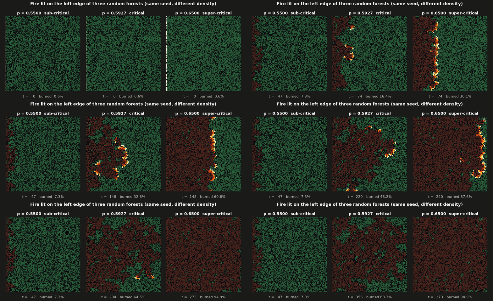
All three forests come from the same random numbers, and only the density differs. Below $p_c$ the fire dies within a few dozen steps. At $p_c$ it crawls along a fractal, dead-end-riddled path (the script picks the first seed whose critical fire makes it across, which happens about half the time). Above $p_c$ a nearly straight front sweeps across.
The phase transition and finite-size scaling
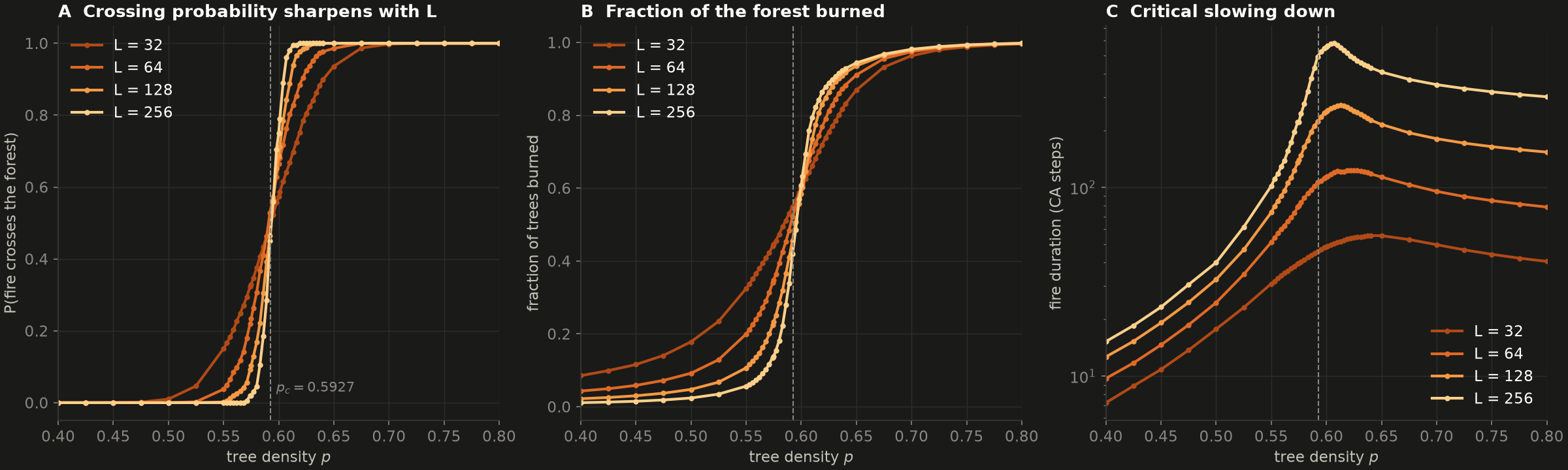
The run uses 2500 / 1200 / 500 / 200 forests for $L$ = 32 / 64 / 128 / 256, over 46 densities that are finest near $p_c$ (steps of 0.003). A. Every curve passes through $P \approx 1/2$ at the same point, and the larger the forest, the steeper the step. B. The burned fraction is the order parameter. For $L\to\infty$ it would be exactly 0 below $p_c$ and would rise with a vertical tangent above it ($\propto (p-p_c)^{5/36}$). C. Fires last longest at $p_c$ (critical slowing down), and the peak grows with $L$.
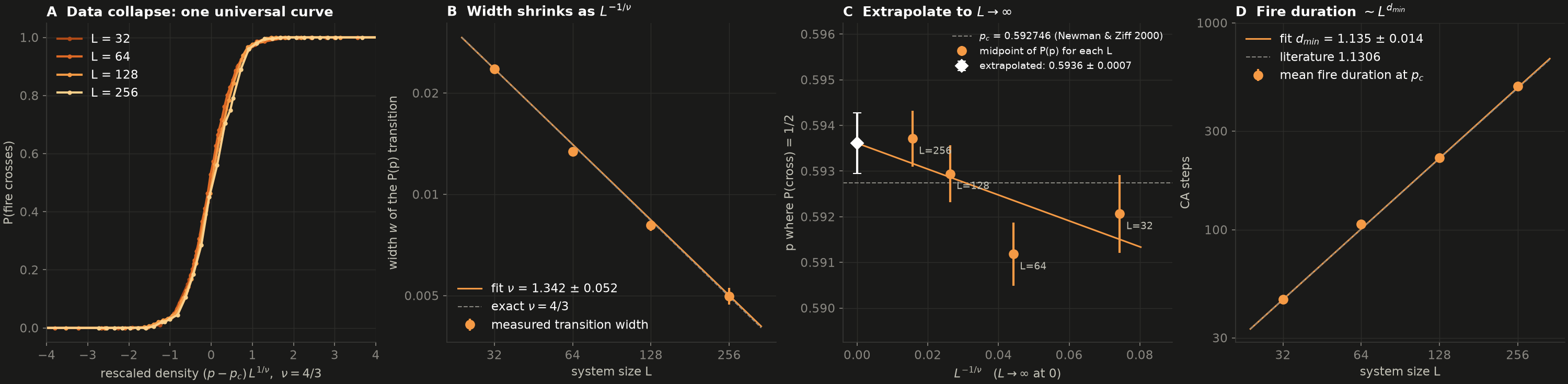
A. Plotted against $(p-p_c)L^{3/4}$, all four sizes fall on one curve: finite-size scaling in one picture. B. The transition width shrinks as $L^{-1/\nu}$. C. The midpoints $p_{1/2}(L)$, extrapolated linearly in $L^{-1/\nu}$ to $L = \infty$, give $p_c$. Note the y-axis: the whole panel spans ±0.0035. D. At $p_c$ the fire duration grows as $L^{d_{min}}$, the fractal dimension of shortest paths.
Part B: self-organised criticality
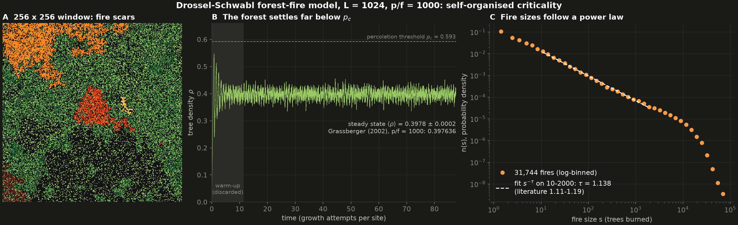
Light green trees are young (grown within the last 0.3 regrowth times, where one regrowth time $N/ heta$ strikes is enough growth attempts to touch every site once), dark green trees are old, and bright patches are fires cooling to ash. The forest becomes a patchwork of fire scars of every size. B. After a transient the density fluctuates around $\langle\rho\rangle \approx 0.398$, far below $p_c = 0.593$. The forest never gets near the percolation threshold, yet C. fire sizes follow a power law over three decades, with a bump and then a cutoff near $10^4$ trees set by $\theta$.
Verification (all numbers from the default run)
| Check | This run | Reference | Result |
|---|---|---|---|
| Front-based CA vs dense textbook CA (3 forests, 64², p = 0.5, p_c, 0.7) | identical arrival time in every cell | — | PASS (exact) |
| $p_c$, extrapolated $L \to \infty$ | 0.5936 ± 0.0007 | 0.592746 (Newman & Ziff 2000) | PASS (tolerance ±0.02, asserted), 1.3 σ high |
| $\nu$ from width scaling | 1.342 ± 0.052 | 4/3 exact | PASS (tol. 0.1), 0.2 σ |
| $d_{min}$ from fire duration at p = 0.592 | 1.135 ± 0.014 | 1.1306 (Zhou et al. 2012) | PASS (tol. 0.05), 0.3 σ |
| $P_L(p_c)$, L = 32 / 64 / 128 / 256 | 0.500 / 0.539 / 0.489 / 0.477 | 1/2 (Cardy 1992) | consistent (binomial SE 0.010 / 0.014 / 0.022 / 0.035; worst is L = 64 at 2.7 SE) |
| DS mean density, $\theta = 1000$ | 0.3978 ± 0.0002 | 0.397636 (Grassberger 2002, Table 1) | PASS (tol. 0.005), about 1 σ |
| DS fire-size exponent, fit 10 ≤ s ≤ 2000 | 1.138 | 1.11–1.19 (τ − 1 from the literature τ) | within range |
The ± values are bootstrap standard errors (300 replicates) for Part A, and batch-means standard errors for the DS density.
Honest notes:
- The ±0.02 tolerance for $p_c$ asked for by the plan is generous. The estimate lands 0.0009 from the exact value, 1.3 bootstrap standard errors. The $L=64$ midpoint sits low and pulls the fitted line (panel C). During development a run with about 1.5× more forests landed at 0.5926 ± 0.0006. That is simply the scatter you get at this sample size. The forest counts were cut to keep the default run short.
- The ±0.05 on $\nu$ is honest but wide. Four sizes spanning only a factor of 8 cannot resolve corrections to scaling, and the logistic shape we fit is a convenience, not the true scaling function $\Phi$ (only its midpoint and width are used).
- The DS error bar comes from 20 batch means, which assumes the batches are nearly independent. Grassberger's value comes from much larger lattices, and $L=1024$ is not infinite.
- The DS "power law" is contested, and that is part of the lesson. Grassberger (2002) ran up to 65536² sites and $\theta = 256\,000$. He found that the density keeps creeping upward with $\theta$ (0.3934 at θ = 500, 0.3976 at θ = 1000, 0.4006 at θ = 2000) and does not settle at the long-quoted limit 0.408. He argued that the apparent scaling laws are transients, and conjectured that the true $\theta\to\infty$ density might be $p_c$ itself. Our exponent 1.138 is an effective exponent over a hand-picked range. It matches what everyone measures at this $\theta$, but it is not a proven universal constant.
Run it
From the repo root:
uv run python L01_wildfire_percolation/sim.py
Runtime: about 3 minutes on a lightly loaded machine (single core, since NumPy element-wise code
is single-threaded). That is an estimate: an earlier configuration with about 1.5× more forests took
232 s wall. The logged run below used 380 s of CPU but 32 min of wall-clock time, because other simulations had the
CPU at 100 %. Wall time scales with how busy your machine is, and the results do not change:
every random stream is seeded, so the numbers are identical on every run. Roughly 55 % of the time
goes to the percolation sweep, 15 % to the 1024² Drossel–Schwabl run and 30 % to the hero and the GIFs.
To go faster, lower samples= in sweep().
It writes to output/:
| File | What |
|---|---|
hero.png |
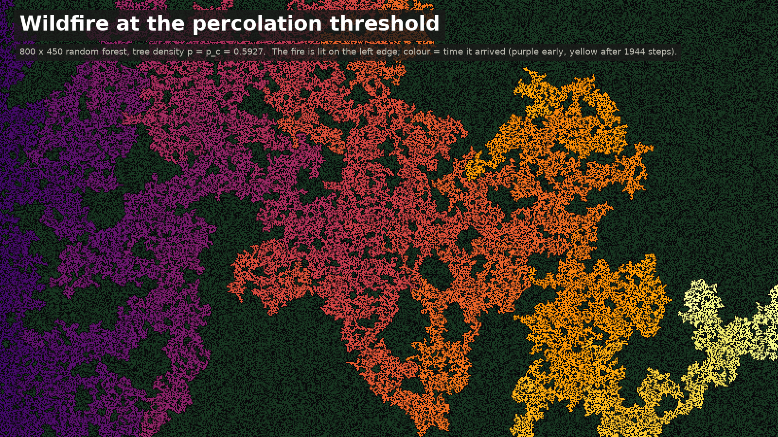
800×450 forest at $p_c$, coloured by fire arrival time |
fire_spread.gif |
three forests (0.55 / $p_c$ / 0.65) burning in lockstep |
percolation_sweep.png |
$P_L(p)$, burned fraction, fire duration |
finite_size_scaling.png |
data collapse, $\nu$, $p_c$ extrapolation, $d_{min}$ |
forest_fire_soc.gif |
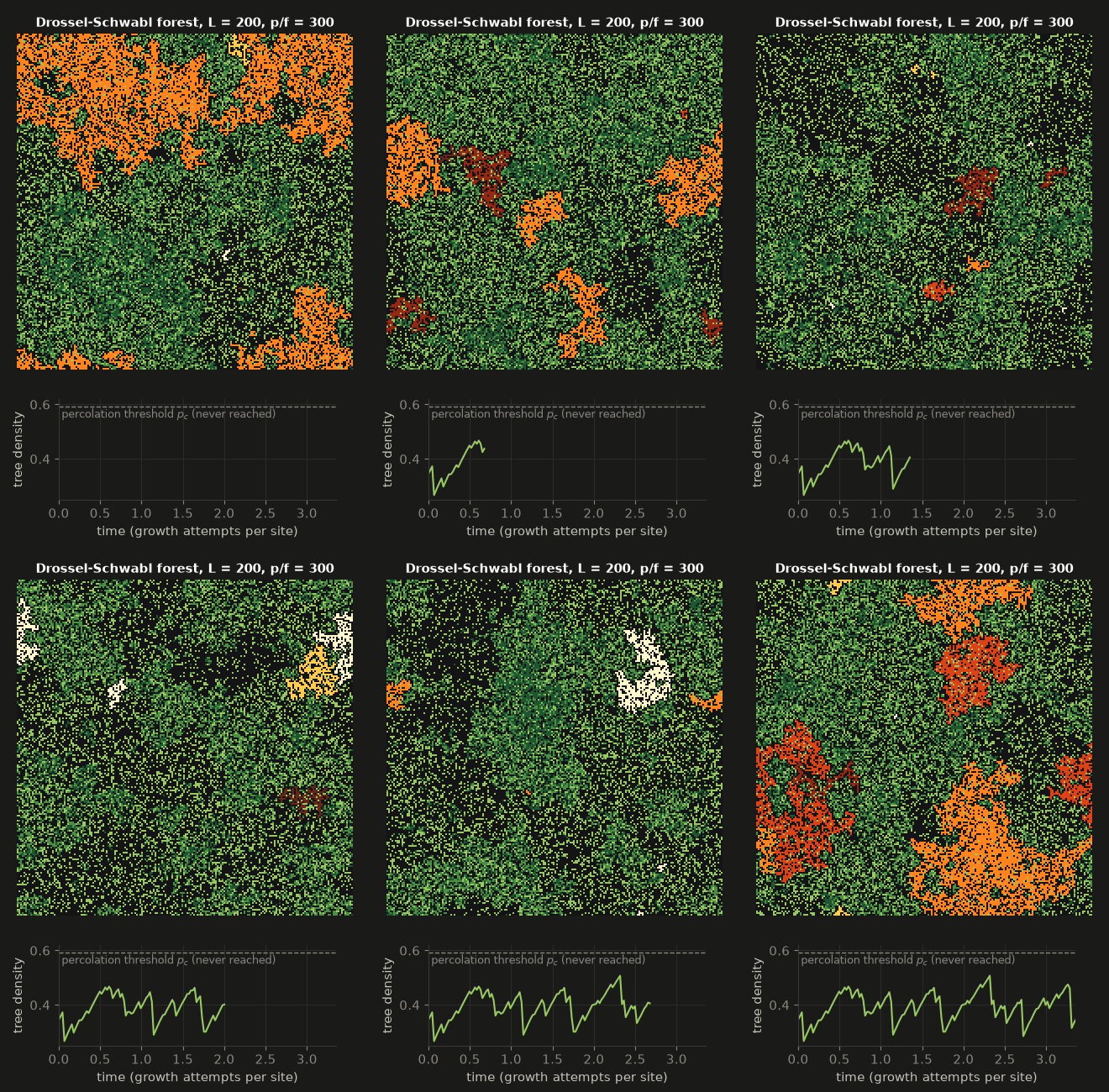
Drossel–Schwabl forest (L = 200, θ = 300) with its density trace |
forest_fire_soc.png |
DS scars, density series, fire-size power law (L = 1024, θ = 1000) |
Console output of the default run
Part A: percolation sweep
  L=  32  S= 2500 forests x 46 densities    42.7 s
  L=  64  S= 1200 forests x 46 densities   165.3 s
  L= 128  S=  500 forests x 46 densities   349.4 s
  L= 256  S=  200 forests x 46 densities   522.3 s
  p_half(L) = [0.5921 0.5912 0.5929 0.5937], width(L) = [0.0236 0.0134 0.0081 0.005 ], duration at p_c = [ 45.9 106.4 223.1 493.9]
  hero: seed 5, fire lasted 1944 steps, burned 50.5% of trees
  Part A done at 1424 s
Part B: Drossel-Schwabl forest fire
  L=1024, p/f=1000: 31744 fires, largest 79616, <rho> = 0.3978, tau = 1.138  (292 s)
  Part B done at 1929 s
Verification
  [PASS] front-based CA reproduces the dense CA exactly
  [PASS] p_c   percolation threshold: 0.5936 +/- 0.0007  expected 0.5927  (tol 0.02)
  [PASS] nu    correlation-length exponent: 1.3415 +/- 0.0515  expected 1.3333  (tol 0.1)
  [PASS] d_min shortest-path dimension: 1.1351 +/- 0.0143  expected 1.1306  (tol 0.05)
  [PASS] rho   DS mean density, p/f=1000: 0.3978 +/- 0.0002  expected 0.3976  (tol 0.005)
  [PASS] tau   DS fire-size exponent: 1.138  literature 1.11-1.19 (an effective exponent, see README)
  P(cross) at p_c: L=32: 0.500, L=64: 0.539, L=128: 0.489, L=256: 0.477   (Cardy 1992: -> 0.5 for a square)
Total runtime 1930 s wall, 380 s CPU    <- machine saturated by other jobs; ~3 min when quiet
Code tour
Everything is in sim.py (about 480 lines, roughly 40 % of them plotting).
| Function | What it does |
|---|---|
spread(trees, front, neighbours) |
The model. A generator that yields successive fire fronts: new front = unburned trees next to the current front, deduplicated with np.unique. It consumes trees in place. Parts A and B both use it, with different neighbour functions. |
arrival_times(trees) |
Pads one forest or a whole batch (S, H, W) with an empty border, lights column 0 and records when each cell ignites. One call burns hundreds of forests at once. |
arrival_times_dense(trees) |
The textbook CA (update every cell every step), kept only as the reference for verification. |
sweep() |
Monte Carlo over $L$ and $p$ with common random numbers. Returns crossing, burned fraction and duration for every forest. |
logistic_fit, estimate, analyse |
Weighted logit fit gives $p_{1/2}(L)$ and $w_L$, then the extrapolation to $p_c$, $\nu$ and $d_{min}$, with 300 bootstrap replicates for the errors. |
drossel_schwabl(L, theta, ...) |
The DS model with a periodic neighbour table (np.roll). Records fire sizes, density per strike and optional RGB frames. |
ds_rgb, fire_rgb |
Map model state to colours (tree age classes, flame → ash ramp). |
power_law(sizes) |
Log-binned $n(s)$ plus a least-squares exponent. |
hero, gif_fire, gif_ds, plot_* |
Figures and animations. The GIF axes are sized so that every cell is exactly 2×2 screen pixels. |
verify(...) |
Cross-checks the two CA implementations and asserts every number in the table above. |
Simplifications & ceilings
- Uniform, isotropic fuel. There is no wind, slope, moisture or fuel type, and the fire always ignites a neighbour (probability 1). Real spread is anisotropic (elliptical fires) and stochastic.
- Four system sizes (32–256) with a linear extrapolation in $L^{-1/\nu}$. Corrections to scaling are ignored. They are small here but would matter at 5-digit precision.
- The front-by-front Python loop costs roughly 20–50 µs per step. That is fine up to about $L = 1000$. For bigger grids use a union-find cluster algorithm (Newman–Ziff) or compile the loop (Numba, L05).
- The DS model runs in the θ-limit only (instantaneous fires), on a modest $1024^2$ grid with $\theta = 1000$. The frontier is $65536^2$ and $\theta \sim 10^5$.
- The power-law fit range (10–2000) is chosen by eye. A rigorous analysis would use maximum likelihood with a data-driven cutoff (Clauset, Shalizi & Newman 2009).
- No real data. Validation is against theory and published simulations, not against observed fires.
Go further
- Wind and flammability. Ignite each neighbour with probability $q$ (bond percolation, $p_c = 1/2$ on the square lattice) and bias $q$ by direction. The fires turn elliptical. Compare their aspect ratio with the Rothermel/Anderson length-to-breadth ratio that FARSITE uses.
- Newman–Ziff. Add trees one at a time with union-find, which gives $P_L(p)$ for all $p$ in one $O(L^2)$ pass. Reach $L = 2048$ and a 5th digit of $p_c$. Compare its cost with this sweep.
- Real fire statistics. Fit the US Fire Program Analysis FPA-FOD wildfire database (Short 2022) and compare the exponent with DS and with Malamud, Morein & Turcotte (1998), who reported power-law fire-size statistics for real US and Australian fires.
- Real fuels. Load a LANDFIRE fuel raster for a Georgia county, set $p$ per cell from fuel load, and compare burn probabilities with FSim's published maps.
- Rebuild it in an industry tool. Write the fire as a NetLogo model (patches plus BehaviorSpace for the sweep), as a Golly rule table, and as a Cadmium Cell-DEVS model. Compare lines of code, run time and how naturally each one expresses the event-driven front.
References
- D. Stauffer & A. Aharony, Introduction to Percolation Theory, 2nd ed., Taylor & Francis (1994).
- K. Christensen & N. R. Moloney, Complexity and Criticality, Imperial College Press (2005).
- M. E. J. Newman & R. M. Ziff, "Efficient Monte Carlo algorithm and high-precision results for percolation", Phys. Rev. Lett. 85, 4104 (2000).
- J. L. Cardy, "Critical percolation in finite geometries", J. Phys. A 25, L201 (1992).
- Z. Zhou, J. Yang, Y. Deng & R. M. Ziff, "Shortest-path fractal dimension for percolation in two and three dimensions", Phys. Rev. E 86, 061101 (2012).
- P. Bak, K. Chen & C. Tang, "A forest-fire model and some thoughts on turbulence", Phys. Lett. A 147, 297 (1990).
- B. Drossel & F. Schwabl, "Self-organized critical forest-fire model", Phys. Rev. Lett. 69, 1629 (1992).
- P. Grassberger, "On a self-organized critical forest-fire model", J. Phys. A 26, 2081 (1993).
- S. Clar, B. Drossel & F. Schwabl, "Forest fires and other examples of self-organized criticality", J. Phys.: Condens. Matter 8, 6803 (1996).
- P. Grassberger, "Critical behaviour of the Drossel–Schwabl forest fire model", New J. Phys. 4, 17 (2002).
- B. D. Malamud, G. Morein & D. L. Turcotte, "Forest fires: an example of self-organized critical behavior", Science 281, 1840 (1998).
- A. Clauset, C. R. Shalizi & M. E. J. Newman, "Power-law distributions in empirical data", SIAM Review 51, 661 (2009).
- R. C. Rothermel, A mathematical model for predicting fire spread in wildland fuels, USDA Forest Service Res. Pap. INT-115 (1972).
- M. A. Finney, FARSITE: Fire Area Simulator — model development and evaluation, USDA Forest Service RMRS-RP-4 (1998).
- G. Wainer, Discrete-Event Modeling and Simulation: A Practitioner's Approach, CRC Press (2009).
- U. Wilensky, NetLogo Fire model, Center for Connected Learning, Northwestern University (1997).