L02 — Noise in Gene Circuits
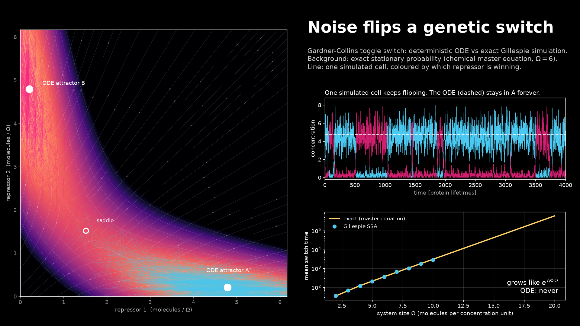
Same genes, same cell, different fate. When a protein is counted in tens of molecules, the textbook ODE is not just imprecise, it is qualitatively wrong: a genetic switch that the ODE says can never flip flips on its own, at a rate that depends exponentially on copy number.
| Toggle switch: 400 identical cells | Repressilator: time-lapse of 100 cells |
|---|---|
 |
 |
1. The question
Deterministic rate equations (ODEs) are the default way to model a chemical or genetic network. They describe concentrations. A real cell holds molecules, and when there are only a few dozen of them, each birth and death of a molecule is a random event.
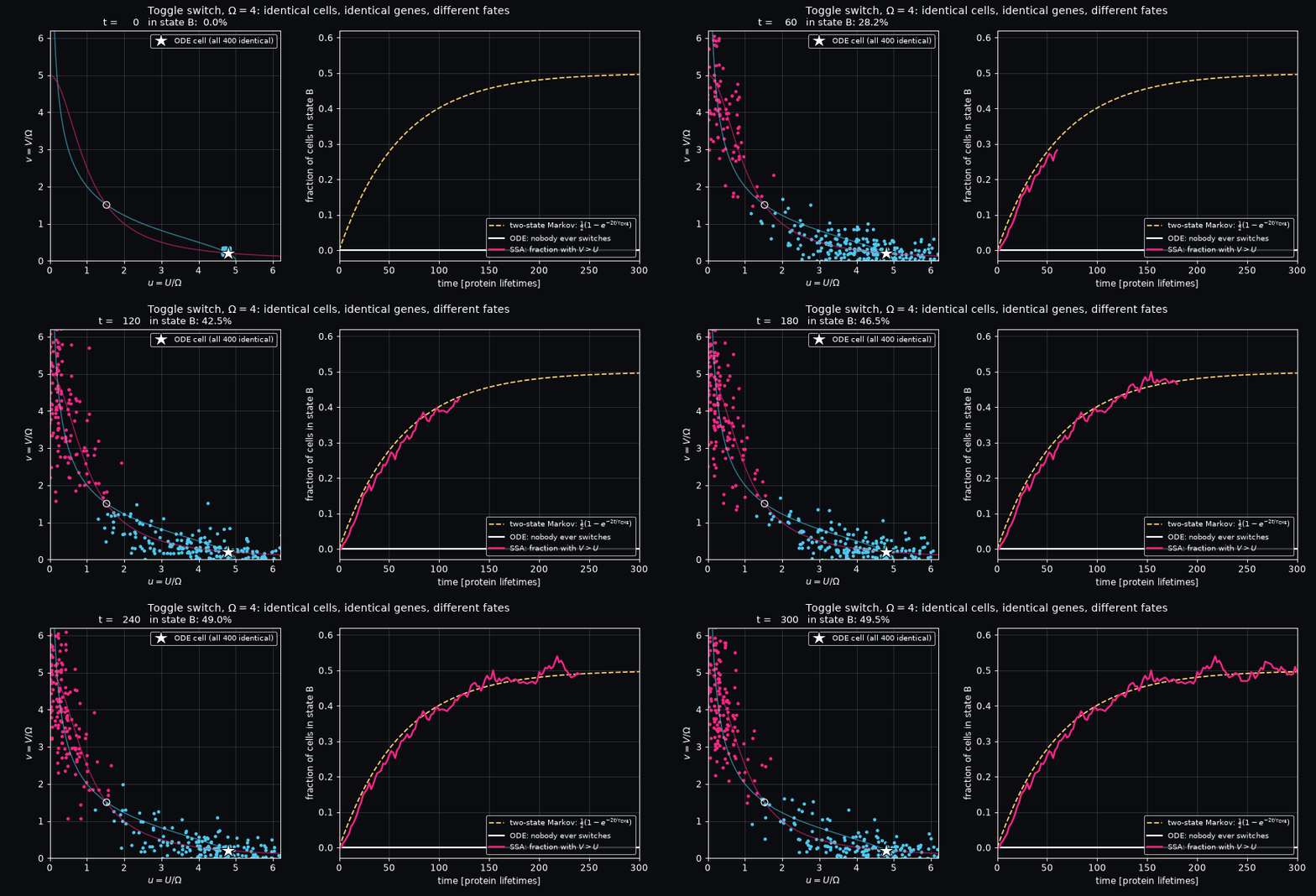
- Toggle switch (Gardner, Cantor & Collins 2000). This bistable circuit is a memory bit. The ODE has two stable states, and a cell that starts in one stays there forever. How often does molecular noise flip it, and how does that rate scale with copy number?
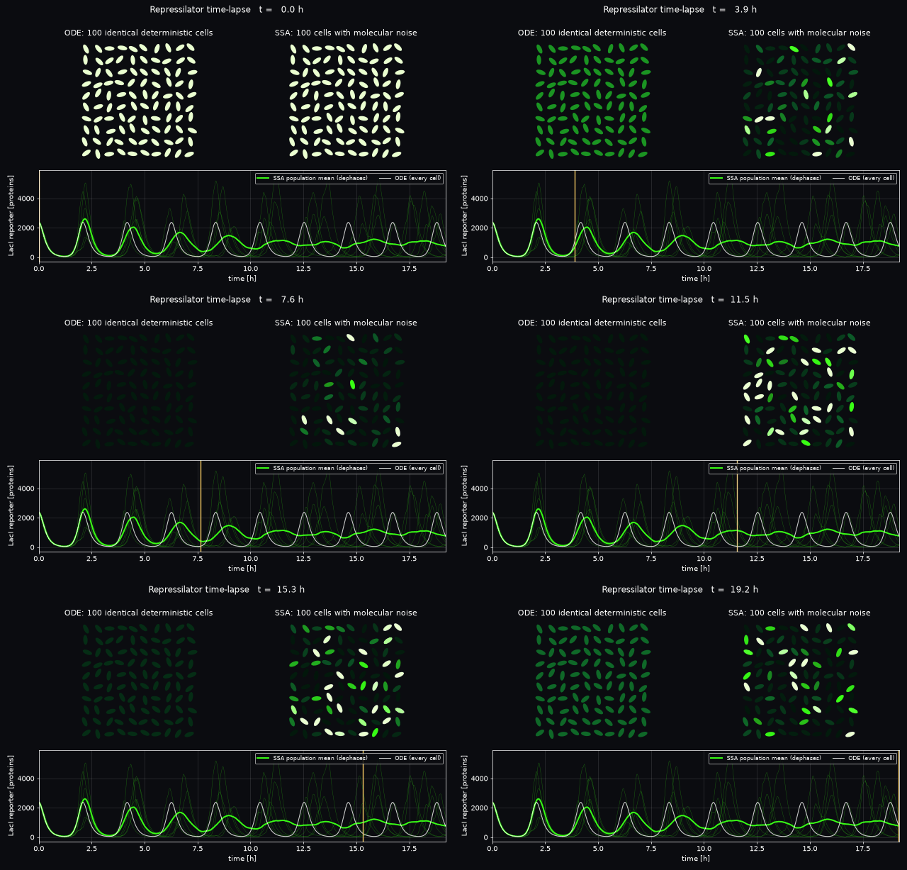
- Repressilator (Elowitz & Leibler 2000). This three-gene ring is a clock. The ODE has a perfect limit cycle. How precise is the clock at the paper's real copy numbers, and how does its precision scale?
- Method questions. How do we simulate the noise exactly (Gillespie SSA)? How do we check that the simulation is right? And which ODE solver should you use when timescales separate (stiffness)?
2. The model
Chemical master equation (CME). Reaction $j$ fires with propensity $a_j(\mathbf{x})$ and changes the state by $\boldsymbol\nu_j$:
$$\frac{\partial P(\mathbf{x},t)}{\partial t}=\sum_j \Big[a_j(\mathbf{x}-\boldsymbol\nu_j)\,P(\mathbf{x}-\boldsymbol\nu_j,t)-a_j(\mathbf{x})\,P(\mathbf{x},t)\Big]$$
Gillespie direct method (SSA) draws exact sample paths of this Markov jump process. In state $\mathbf x$:
- compute every propensity $a_j(\mathbf x)$;
- total rate $a_0=\sum_j a_j$;
- waiting time $\tau \sim \mathrm{Exp}(a_0)$, i.e. $\tau=-\ln(r_1)/a_0$;
- pick reaction $j$ with probability $a_j/a_0$;
- set $\mathbf x \leftarrow \mathbf x+\boldsymbol\nu_j$ and $t\leftarrow t+\tau$, then repeat.
As the system size $\Omega\to\infty$, $\mathbf x/\Omega$ converges to the ODE $\dot{\mathbf c}=\sum_j \boldsymbol\nu_j\,\tilde a_j(\mathbf c)$ (Kurtz 1972). The ODE is therefore the large-number limit of the SSA, not the other way round.
| Model | ODE (dimensionless) | Reactions (counts) | Parameters |
|---|---|---|---|
| Birth–death (verification) | $\dot x = k-\gamma x$ | $\varnothing\xrightarrow{k}X$, $X\xrightarrow{\gamma x}\varnothing$ | $k=10,\ \gamma=1$. Exact law: Poisson$(\tfrac{k}{\gamma}(1-e^{-\gamma t}))$ |
| Toggle switch | $\dot u=\frac{\alpha}{1+v^n}-u,\ \ \dot v=\frac{\alpha}{1+u^n}-v$ | $\varnothing\to U$ at $\Omega\alpha/(1+(V/\Omega)^n)$, $U\to\varnothing$ at $U$, and the same with $U\leftrightarrow V$ | $\alpha=5,\ n=2$. Time in protein lifetimes. $\Omega$ = molecules per concentration unit |
| Repressilator | $\dot m_i=-m_i+\frac{\alpha}{1+p_{i-1}^n}+\alpha_0,\ \ \dot p_i=-\beta(p_i-m_i)$ | 12 reactions: transcription, mRNA decay, translation, protein decay | $\alpha=216,\ \alpha_0=0.216,\ \beta=0.2,\ n=2$ (paper, Box 1). Time unit = mRNA lifetime = 2.885 min |
Repressilator copy numbers. These come from the paper's own figures: $K_M=40$ repressor monomers per cell, 20 proteins per transcript, and protein/mRNA half-lives of 10/2 min. So one unit of $p$ is 40 proteins and one unit of $m$ is 0.4 mRNAs, and translation fires at $20\,M$ per mRNA lifetime. A scale factor $s$ multiplies both; $s=1$ is the paper's cell.
Exact alternative for the toggle. On the lattice $0\le U,V\le N$ the CME is a sparse linear system $\dot P = Q^\top P$ (finite state projection; Munsky & Khammash 2006). The stationary law solves $Q^\top\pi=0$. The mean first-passage time $h(\mathbf x)$ into the other state's basin $B=\{V-U\ge\delta\Omega\}$ solves $Q h=-1$ off $B$, with $h=0$ on $B$. These are two spsolve calls, and they give an independent exact answer to check the SSA against.
Assumptions. The cell is well mixed. The promoter is quasi-steady, so the Hill function sits directly in the propensity. Dilution is lumped into degradation. There is no cell division, no extrinsic noise, and no spatial structure.
3. M&S concepts you'll learn here
- Deterministic vs stochastic models. The ODE is the $\Omega\to\infty$ limit of the CME (Kurtz), and it fails qualitatively for rare events such as switching.
- Chemical master equation and Gillespie SSA. An exact sampler of a continuous-time Markov chain needs only two random numbers per event.
- Vectorising Monte Carlo across replicas. Each NumPy loop iteration advances every cell by one event, each on its own clock (~2–6 M events/s in plain NumPy).
- Markov property as a tool. A long run can be cut into chunks and restarted from the last state exactly, which keeps memory bounded.
- Exact CME solves by sparse linear algebra (finite state projection): stationary distributions and mean first-passage times without any sampling noise.
- Rare events and large deviations. The switching time grows like $e^{\Delta\Phi\,\Omega}$, the chemical analogue of the Arrhenius/Kramers law, and waiting times are memoryless.
- Censored data. The exponential MLE $\hat\tau=\sum_i\min(T_i,t_{\max})/\#\text{hits}$ uses the runs that did not finish too.
- Bistability analysis. Nullclines, fixed points by bracketing plus
brentq, and stability from Jacobian eigenvalues. - Limit cycles and phase diffusion. Noise turns a sharp spectral line into a broadened peak, and the period CV scales like $\Omega^{-1/2}$ (linear noise approximation), but only once copy numbers are large enough.
- Stiffness. Explicit Runge–Kutta cost grows with the fast/slow timescale ratio; implicit BDF/Radau and auto-switching LSODA stay flat.
- Verification ladder. Check against an exact analytic law (Poisson), then against an independent exact numerical method (CME), then validate against experiment (Elowitz's measured period).
4. Tech stack
| Tool | Role here |
|---|---|
| Python 3.12 | everything |
| NumPy | the vectorised Gillespie engine, histograms, fits |
| Matplotlib (+ Pillow) | figures and GIF animations (FuncAnimation + PillowWriter) |
★ SciPy integrate.solve_ivp |
the ODE models; RK45 / DOP853 / LSODA / BDF / Radau benchmark |
★ SciPy optimize.brentq |
toggle fixed points (bracketed root finding) |
★ SciPy sparse + sparse.linalg.spsolve |
exact CME: stationary law and mean first-passage times on up to 36 000 states |
★ SciPy signal.find_peaks, fft |
repressilator peak-to-peak periods and power spectra |
★ SciPy stats |
Poisson pmf and the χ² goodness-of-fit test for SSA verification |
★ SciPy ndimage.zoom |
smoothing the lattice landscape for display |
multiprocessing.Pool (stdlib) |
4 worker processes for the independent SSA runs |
SciPy matters because it turns NumPy arrays into numerical methods: adaptive and stiff integrators, root finders, sparse direct solvers and signal processing. Each of these would be a project to write yourself.
5. Industry & scientific tools
| Tool | What it is | Who uses it | How this project maps to it |
|---|---|---|---|
| COPASI | GUI and engine for biochemical networks: ODE (LSODA), SSA, hybrid, parameter estimation | systems-biology labs, teaching | the same ODE-vs-SSA comparison is two clicks in COPASI; its LSODA is the solver benchmarked here |
| Tellurium / libRoadRunner | Python environment with a fast C++ SBML simulator (CVODE, Gillespie) | synthetic-biology design (Sauro lab and others) | te.loada(antimony).gillespie() replaces gillespie(); the model is the same Antimony/SBML |
| SBML | the XML exchange standard for reaction networks | every tool here; BioModels database | our stoich + propensity pairs are exactly an SBML reaction list |
| GillesPy2 / StochKit2 / StochSS | optimised SSA, tau-leaping and hybrid solvers (C++ back-ends) | stochastic cell-biology modelling | same direct method, compiled; tau-leaping is the next step for big networks |
| BioNetGen | rule-based modelling that generates huge reaction networks | signalling and immunology | for combinatorial networks where writing reactions by hand is impossible |
| MATLAB SimBiology | commercial model builder with ODE and SSA solvers | pharma (PK/PD, QSP) | same ODE/SSA dichotomy, in industry drug-development workflows |
| Smoldyn / MCell | particle-based spatial stochastic simulators | neuroscience synapses, membrane signalling | drops our well-mixed assumption |
6. Results
Verification first: the SSA reproduces an exact law
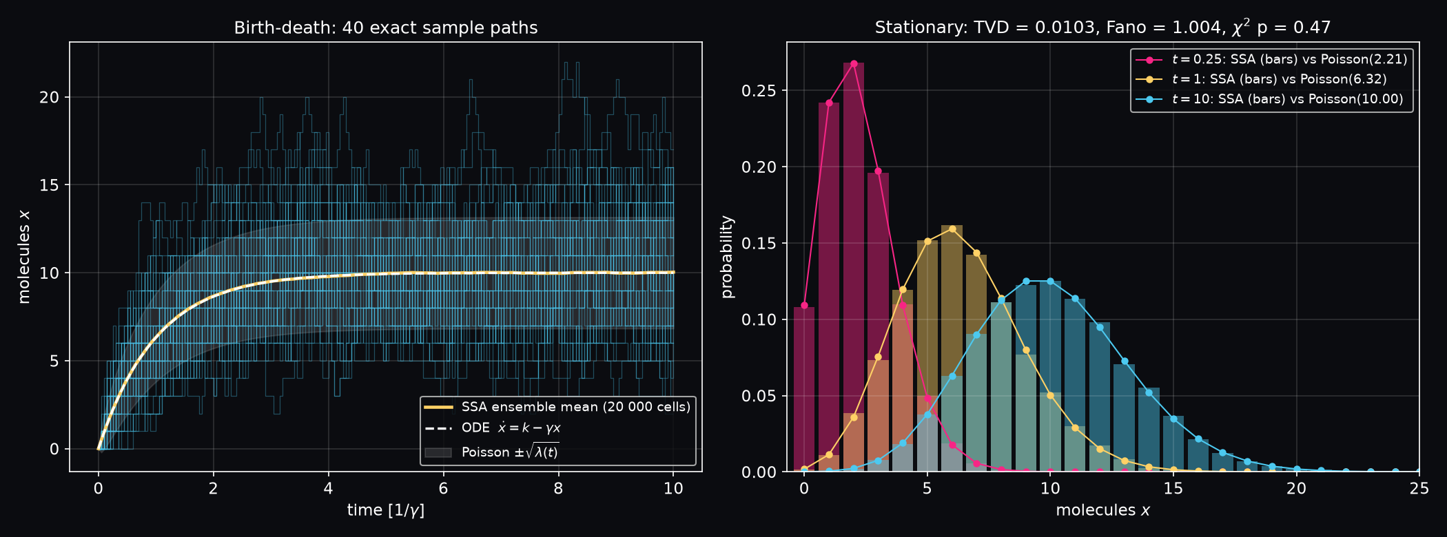
Started from $x=0$, the birth–death process has the law Poisson$(\lambda(t))$ at every time. The SSA matches it along the whole transient (right panel), not just at the mean.
Toggle switch: the ODE never flips, the cell does
- ODE fixed points (from
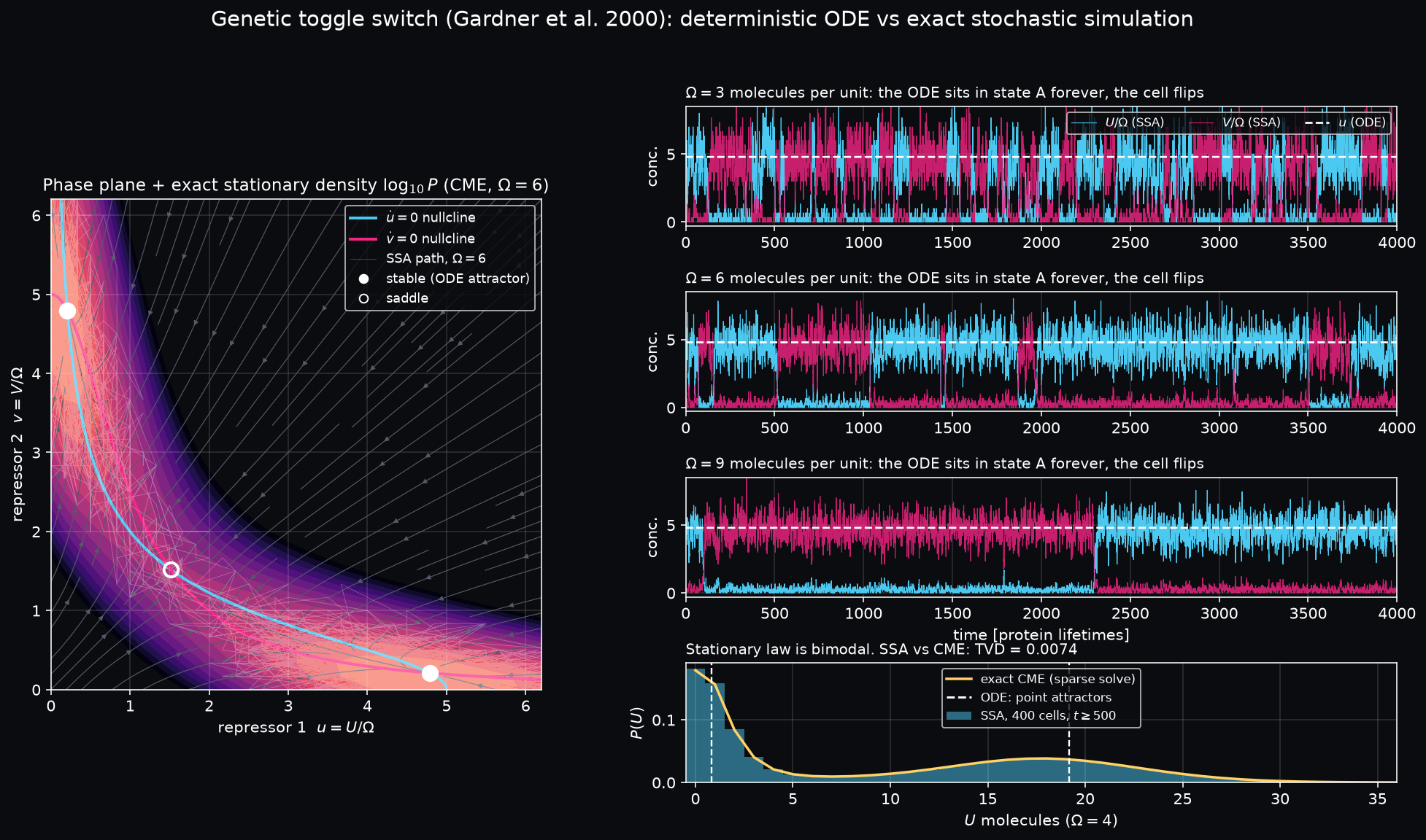
brentqplus Jacobian eigenvalues): stable A = (4.791, 0.209), saddle (1.516, 1.516), stable B = (0.209, 4.791). Started in A, the ODE stays at $u=4.791$ for all time. This is guaranteed: A is asymptotically stable and ODE solutions are unique. - The SSA at the same parameters hops between A and B. At $\Omega=3$ it is a noisy telegraph signal, at $\Omega=6$ it flips every few hundred lifetimes, and at $\Omega=9$ only twice in 4000.
- The stationary law of $U$ at $\Omega=4$ is bimodal. The ODE instead predicts two point attractors, and which one you get depends only on the initial condition.
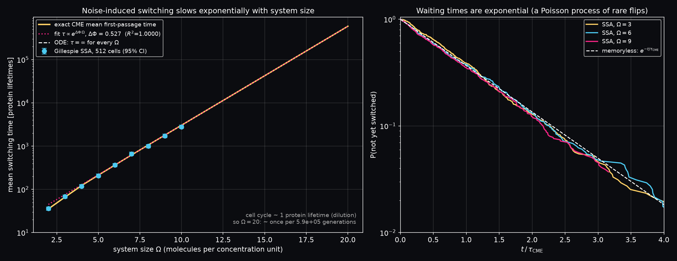
Mean switching time, SSA (512 cells per Ω, censored MLE, 95% CI) vs the exact CME answer:
| Ω | 2 | 3 | 4 | 5 | 6 | 7 | 8 | 9 | 10 |
|---|---|---|---|---|---|---|---|---|---|
| SSA τ̂ | 36.1 | 68.2 | 118.3 | 206.7 | 365.9 | 665.1 | 999.8 | 1725 | 2790 |
| CME exact | 35.4 | 66.4 | 123.1 | 213.6 | 365.8 | 627.0 | 1061.5 | 1798 | 3045 |
| z-score | +0.42 | +0.60 | −0.90 | −0.74 | +0.01 | +1.30 | −1.35 | −0.92 | −1.95 |
The CME extends the curve where sampling becomes hopeless: τ = 5.9×10⁵ protein lifetimes at Ω = 20. A fit over Ω ≥ 10 gives $\ln\tau = 2.751 + 0.5271\,\Omega$ with $R^2 = 1.00000$. That is pure exponential scaling, with effective barrier ΔΦ ≈ 0.527 per unit of Ω. Since protein lifetime ≈ cell cycle (dilution), a switch with ~20 molecules per concentration unit is epigenetic memory that lasts ~10⁵–10⁶ generations. At ~5 it forgets within a few hundred. The survival curves (right) are straight lines on a log axis: flips are memoryless, which is why the two-state Markov curve fits the population GIF.
Repressilator: the clock is noisy, and its period drifts with copy number
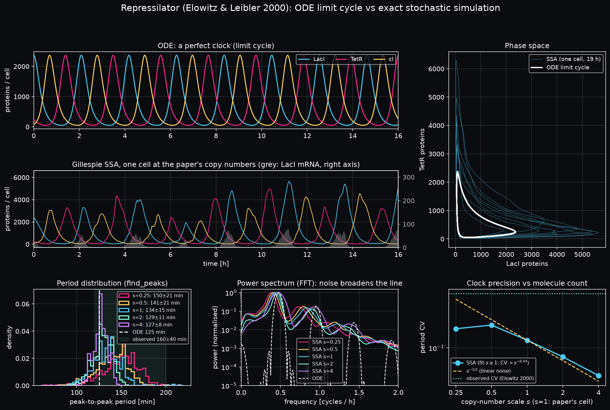
- ODE: period 43.45 mRNA lifetimes = 125.4 min, with LacI peaking at 59.2 $K_M$ ≈ 2370 proteins. Elowitz & Leibler measured 160 ± 40 min (mean ± s.d.). The ODE lands inside one standard deviation using only the paper's biochemical parameters, with no fitting.
- SSA at the paper's copy numbers ($s=1$; mRNA is often only 0–5 molecules): period 133.5 ± 15.2 min (CV 0.114, 709 peak-to-peak intervals from 100 cells over 19 h). The FFT peak is at 140.1 min. Noise does more than blur the clock. It lengthens the period and raises the peaks (mean LacI peak 80.1 vs the ODE's 59.2 $K_M$), because a repressor that stochastically drains to zero lets the next gene overshoot.
- The ODE is the large-copy-number limit (Kurtz). As $s$ grows, every SSA statistic walks toward the ODE:
| scale $s$ | 0.25 | 0.5 | 1 (paper) | 2 | 4 | ODE |
|---|---|---|---|---|---|---|
| mean period [min] | 149.6 | 140.8 | 133.5 | 129.4 | 127.2 | 125.4 |
| period s.d. [min] | 20.7 | 20.7 | 15.2 | 11.1 | 8.0 | 0 |
| period CV | 0.138 | 0.147 | 0.114 | 0.086 | 0.063 | 0 |
| FFT peak period [min] | 156.7 | 146.7 | 140.1 | 130.2 | 128.6 | 125.4 |
| mean LacI peak [$K_M$] | 123.4 | 99.0 | 80.1 | 70.9 | 64.6 | 59.2 |
- Clock precision. The linear noise approximation predicts CV $\propto s^{-1/2}$. The fit over $s\ge1$ gives $s^{-0.432}$. Honest miss: the first version of this script fit all five scales and got $s^{-0.306}$, which fails the ±0.15 test. Below $s\approx1$ the CV saturates near 0.14, because mRNA sits at 0–1 molecules for much of the cycle and the small-noise expansion is invalid. The test now checks the law only where the theory applies, and both numbers are printed.
- Validation gap. The measured CV of 0.25 is about twice the simulated 0.114. Intrinsic noise alone does not explain the experiment. Cell division, plasmid-copy variation and extrinsic noise are missing (see Simplifications).
- The time-lapse GIF shows it at the population level. Identical cells start in phase, the ODE colony blinks in lock-step forever, and the SSA colony dephases over ~10–20 h. The population mean decays even though every single cell keeps oscillating.
Stiff vs non-stiff ODE solvers
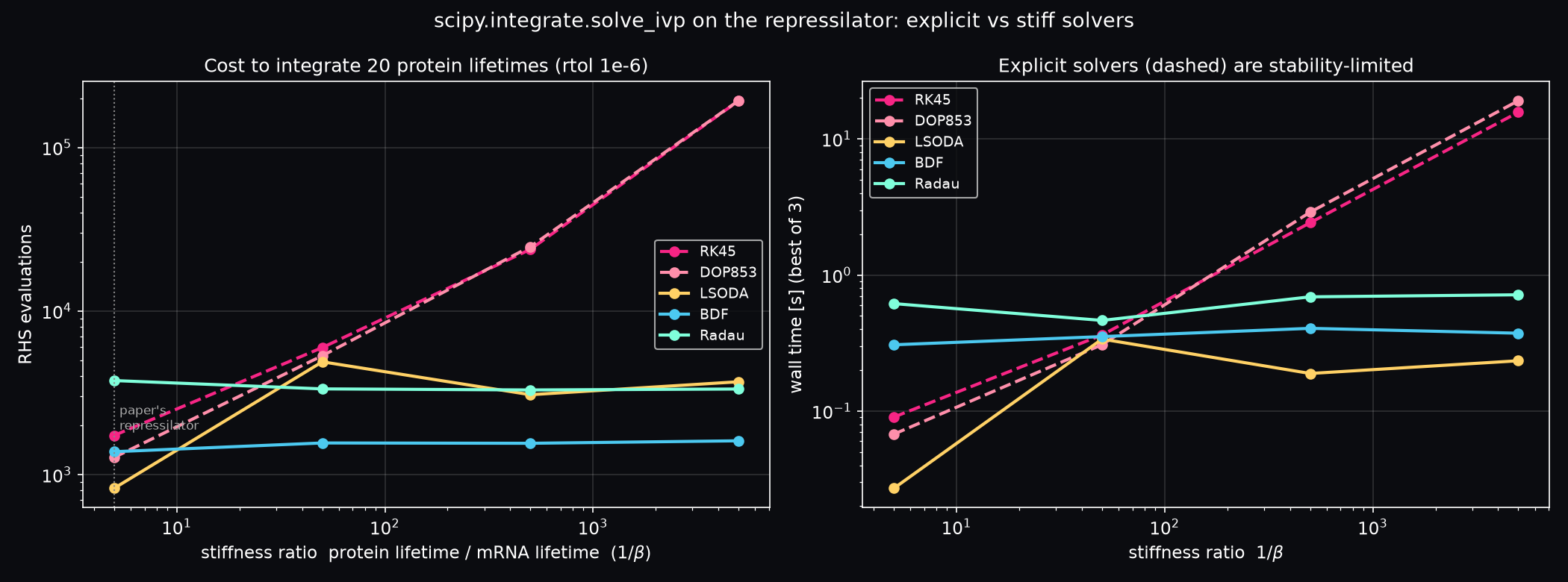
Stiffness knob: protein lifetime / mRNA lifetime $=1/\beta$. The paper's value is 5; real proteins that are diluted by growth give 20–100+. Each run integrates 20 protein lifetimes at rtol=1e-6, and errors are measured against Radau at rtol=1e-11.
| ratio $1/\beta$ | RK45 fevals (s) | DOP853 fevals (s) | LSODA fevals (s) | BDF fevals (s) | Radau fevals (s) |
|---|---|---|---|---|---|
| 5 (paper) | 1 736 (0.090) | 1 274 (0.068) | 825 (0.027) | 1 380 (0.31) | 3 758 (0.62) |
| 50 | 5 978 (0.36) | 5 330 (0.31) | 4 893 (0.34) | 1 561 (0.35) | 3 342 (0.46) |
| 500 | 23 846 (2.4) | 24 758 (2.9) | 3 079 (0.19) | 1 554 (0.41) | 3 292 (0.69) |
| 5000 | 192 734 (15.7) | 193 202 (19.1) | 3 695 (0.23) | 1 609 (0.37) | 3 336 (0.72) |
- On the non-stiff paper model, explicit RK45/DOP853 are fine. The implicit methods pay for Jacobians and linear solves, so they are 3–7× slower even though their feval counts are similar.
- As the timescales separate, explicit cost grows roughly linearly with the stiffness ratio: the step size is capped by stability (the fast mRNA), not by accuracy. BDF/Radau stay flat at ~1.5–3.7k evaluations. At ratio 5000, LSODA is 67× faster than RK45 in wall time (52× fewer evaluations).
- LSODA detects stiffness and switches between Adams and BDF on its own. That is why it is COPASI's default, and it is the right first choice. All relative errors are ≤ 1e-5 except LSODA at ratio 50 (2.1e-4). That case is a damped oscillation where a small phase error shows up as amplitude error, a reminder that
rtolis a local per-step tolerance, not a guarantee on the global error. - Seconds are wall-clock on a shared, fully loaded machine. The evaluation counts are the reproducible numbers.
Verification & validation summary (actual printed values)
| Check | Expected | Got | |
|---|---|---|---|
| Birth–death mean (20 000 cells at t = 10) | k/γ(1−e⁻¹⁰) = 9.9995 ± 0.022 | 10.037 | PASS |
| Birth–death Fano factor (var/mean) | 1 (Poisson) | 1.004 | PASS |
| Birth–death χ² goodness of fit vs Poisson | p > 0.001 | χ² = 18.8 / 19 dof, p = 0.473 | PASS |
| Birth–death total-variation distance | → 0 | 0.0103 | PASS |
| Toggle ODE fixed points | 2 stable + 1 saddle | 2 + 1 | PASS |
| Toggle stationary P(U), SSA vs exact CME, Ω = 4 | TVD → 0 | 0.0074 | PASS |
| Toggle mean switching time, SSA vs exact CME, Ω = 2…10 | |z| < 3 for all | max |z| = 1.95 | PASS |
| Toggle ln τ linear in Ω (CME, Ω ≥ 10) | R² > 0.999 | R² = 1.00000, slope 0.5271 | PASS |
| Repressilator ODE period vs experiment (Elowitz 2000) | 160 ± 40 min | 125.4 min | PASS |
| Repressilator SSA → ODE (Kurtz), s = 4 | within 5% of 125.4 min | 127.2 min (+1.4%) | PASS |
| Repressilator period CV ∝ s^−1/2 (LNA), s ≥ 1 | −0.50 ± 0.15 | −0.432 | PASS |
| (reported, not asserted) the same fit over all s | −0.50 | −0.306 | miss, see above |
7. Run it
# from SimulationLab/
uv run python L02_gene_circuit_noise/sim.py
Runtime. The first full run with a comparable workload took 3.6 min (218 s) on the 8-core dev machine, using 4 worker processes for the SSA batch. The final run that produced the numbers above took 12.7 min (760 s), because other simulations had the machine at 100% CPU: the same RK45 solve was 5.6× slower. Expect about 3.5–4 min on an idle machine. All randomness is seeded (SEED = 2000, one stream per job), so the toggle and birth–death numbers are bit-for-bit reproducible. Only the wall-clock solver timings vary.
Outputs go to output/: hero.png, birth_death_verification.png, toggle_ode_vs_ssa.png, toggle_switching_time.png, repressilator.png, solver_benchmark.png, toggle_population.gif, repressilator_cells.gif. The script ends with a PASS/FAIL table and raises AssertionError if any check fails.
8. Code tour (sim.py)
| Function | What it does |
|---|---|
gillespie(x0, stoich, propensity, t_end, dt, rng) |
the algorithm: the direct method, 5 commented steps, vectorised over cells, state sampled on a regular grid |
bd_propensity, toggle_propensity(Ω), repressilator_propensity(s) |
reaction rates; each model is just a stoichiometry matrix plus a propensity function |
toggle_rhs, repressilator_rhs |
the deterministic counterparts for solve_ivp |
toggle_fixed_points |
nullcline intersection by sign-change bracketing plus brentq, and stability from Jacobian eigenvalues |
toggle_cme, cme_mfpt, cme_stationary |
sparse CME generator; exact first-passage times (Q h = −1) and stationary law (Qᵀπ = 0) |
toggle_fpt_job |
SSA first-passage times A→B in 1000-unit chunks (Markov restart), censored at 3·τ_CME |
ssa_job |
picklable wrapper so multiprocessing.Pool can run any model |
birth_death |
verification against Poisson (mean, Fano, χ², TVD) and its figure |
rep_ode_reference, rep_periods, spectrum |
limit-cycle state and period; peak-to-peak intervals; Hann-windowed, zero-padded FFT |
solver_benchmark |
RK45 / DOP853 / LSODA / BDF / Radau across stiffness ratios 5…5000 against a tight Radau reference |
main |
the whole pipeline: verify → toggle → repressilator → 4-process SSA batch → analyses → benchmark → PASS/FAIL table |
fig_*, gif_*, make_hero |
plotting only |
9. Simplifications & ceilings
- No promoter states, no bursts in the toggle. The Hill function goes straight into the propensity, which is a stochastic quasi-steady-state assumption. With explicit operator binding and mRNA, the switching rate changes, sometimes by orders of magnitude.
- Intrinsic noise only. No cell division, partitioning noise or cell-to-cell parameter spread (extrinsic noise). This is the main reason the simulated period CV (≈0.11) sits below the measured one (0.25).
- Engine speed. The vectorised NumPy SSA does ~2–6 M events/s per process (more cells per loop means more events/s). The cost of the toggle study grows like $\Omega\,e^{0.53\Omega}$, so SSA stops at Ω = 10 and the CME takes over. Upgrade paths: Numba (L05), the Gibson–Bruck next-reaction method for large networks, tau-leaping for high copy numbers, and rare-event samplers (forward-flux or weighted-ensemble) for Ω ≫ 10.
- First-passage times are detected on a grid (dt = 0.25, corrected by −dt/2), marked
ponytail:in the code. An exact per-event hit test would remove the ±0.125 time-unit error, which is already <0.4% of τ. - The CME is truncated at $N=\alpha\Omega+8\sqrt{\alpha\Omega}+10$ molecules. The dropped probability mass is negligible, but the method only works while the state space fits (2 species × ~200 states each). A 6-species repressilator would need ~10¹² states, which is exactly why SSA exists.
- The censored exponential MLE assumes memoryless flips. The survival plot checks this, and censoring is ~5% (3·τ cut-off).
- Solver timings are wall-clock on a machine shared with other jobs. RHS-evaluation counts are the robust metric; the seconds are indicative.
10. Go further
- Rebuild it in Tellurium or COPASI. Write the toggle in Antimony (
J1: -> U; W*a/(1+(V/W)^2)…), runr.gillespie()over many cells, and check that your MFPT matches the CME numbers above. Export the SBML and open it in COPASI to compare its LSODA against oursolve_ivp. - Chemical Langevin / tau-leaping. Replace exact SSA with the CLE and measure the switching time at Ω = 6–10. Diffusion approximations are known to get rare-event rates exponentially wrong. Quantify by how much.
- Predict ΔΦ from theory. Compute the WKB quasi-potential with a minimum-action path (geometric minimum action method,
scipy.optimize.minimizeon a discretised path) and compare with the fitted slope 0.527. - Add biology. Give the toggle explicit mRNA and promoter states (bursty expression), or add cell division with binomial partitioning to the repressilator. Does the CV approach Elowitz's 0.25?
- Reproduce Gardner's experiment. Add an inducer that transiently lowers α₁ (an IPTG pulse), map the hysteresis loop in the ODE, and measure how noise shrinks the bistable window.
11. References
- D. T. Gillespie, "Exact stochastic simulation of coupled chemical reactions," J. Phys. Chem. 81, 2340 (1977); and J. Comput. Phys. 22, 403 (1976).
- T. S. Gardner, C. R. Cantor, J. J. Collins, "Construction of a genetic toggle switch in Escherichia coli," Nature 403, 339 (2000).
- M. B. Elowitz, S. Leibler, "A synthetic oscillatory network of transcriptional regulators," Nature 403, 335 (2000).
- T. G. Kurtz, "The relationship between stochastic and deterministic models for chemical reactions," J. Chem. Phys. 57, 2976 (1972).
- B. Munsky, M. Khammash, "The finite state projection algorithm for the solution of the chemical master equation," J. Chem. Phys. 124, 044104 (2006).
- P. Gaspard, "The correlation time of mesoscopic chemical clocks," J. Chem. Phys. 117, 8905 (2002).
- M. A. Gibson, J. Bruck, "Efficient exact stochastic simulation of chemical systems with many species and many channels," J. Phys. Chem. A 104, 1876 (2000).
- D. T. Gillespie, "Approximate accelerated stochastic simulation of chemically reacting systems" (tau-leaping), J. Chem. Phys. 115, 1716 (2001).
- M. B. Elowitz, A. J. Levine, E. D. Siggia, P. S. Swain, "Stochastic gene expression in a single cell," Science 297, 1183 (2002).
- N. G. van Kampen, Stochastic Processes in Physics and Chemistry, 3rd ed. (Elsevier, 2007).
- D. J. Wilkinson, Stochastic Modelling for Systems Biology, 3rd ed. (CRC Press, 2018).
- E. Hairer, G. Wanner, Solving Ordinary Differential Equations II: Stiff and Differential-Algebraic Problems (Springer, 1996).