L04 — Echo Chambers
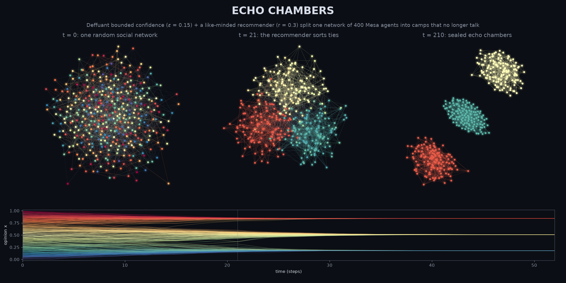
Give 400 simulated people a limited tolerance for disagreement and a friend recommender, and one random social network splits into sealed camps that no longer talk to each other.
The question
Where do echo chambers come from? Two mechanisms are usually blamed:
- Bounded confidence. People are only persuaded by views that are already fairly close to their own.
- Selective exposure. Platforms (and people) drop ties to those who disagree and suggest like-minded ones instead.
This level builds an agent-based model (ABM) with both mechanisms turned into dials. It then asks: which dial decides how many opinion camps form, and which one decides whether the camps stay in contact? A parallel sweep over both dials gives a phase diagram: consensus / polarisation / fragmentation, with the network-level echo-chamber boundary drawn on top.
Why agent-based? (versus L02's ODEs and L03's DES)
| L02 ODE / SSA | L03 discrete-event | L04 agent-based | |
|---|---|---|---|
| State | a few population-level concentrations | queues, servers and entities flowing through a fixed process | every individual's own state (here: an opinion in [0, 1]) |
| Who interacts with whom | well-mixed: mass action | entities meet resources, not each other | local: only along network ties |
| Heterogeneity | averaged away | entity attributes, but the process is shared | the point of the model: 400 different opinions and neighbourhoods |
| Structure | fixed equations | fixed flowchart | adaptive: agents rewire the network, and the network steers the agents |
| What you get out | trajectories you could often derive | throughput and waiting-time statistics | emergent macro patterns (camps, chambers) that no rule mentions |
Nothing in the agent rules says "form three groups" or "split the network". Both are emergent: they appear only from many local interactions. This is also why an ABM needs many replications and a parameter sweep. A single run is one draw from a distribution of possible societies.
The model (ODD, compact)
Agent-based models in research papers are documented with the ODD protocol (Overview, Design concepts, Details; Grimm et al. 2006, 2020). ODD is a fixed checklist, so another group can re-implement your model without reading your code. Here is this model in ODD form:
Overview
- Purpose: test whether opinion-driven tie rewiring (a "recommender") turns opinion clusters into
disconnected echo chambers, and whether it changes how many clusters form.
- Entities and state variables: Person agents, each with an opinion $x_i \in [0,1]$ and fixed to a
node of an undirected network. Global parameters: confidence bound $\varepsilon$, convergence rate $\mu$,
rewiring probability $r$.
- Scales: $N = 400$ agents on a $G(n, m)$ random graph with mean degree $\langle k \rangle = 12$
(2400 ties). Time is in steps. One step means every agent acts once, in random order (asynchronous
random-sequential updating). A run stops at convergence or after 600 steps.
- Process overview: each activated agent $i$ picks a random neighbour $j$ and then:
$$ |x_j - x_i| < \varepsilon:\quad x_i \leftarrow x_i + \mu (x_j - x_i),\;\; x_j \leftarrow x_j - \mu (x_j - x_i) \qquad \text{(Deffuant et al. 2000)} $$
$$ |x_j - x_i| \ge \varepsilon:\quad \text{with prob. } r,\ \text{drop tie } (i,j),\ \text{add tie } (i,k) \text{ to a stranger } k \text{ with } |x_k - x_i| < \varepsilon $$
Design concepts - Emergence: the number of opinion clusters, the network modularity and the number of network components. - Adaptation / interaction: pairwise, along ties only. The recommender samples up to 20 random strangers and returns the first one within $\varepsilon$ that is not already a neighbour. - Stochasticity: initial graph, initial opinions $x_i \sim U(0,1)$, activation order, partner choice, rewiring. The same seeds are used in every sweep cell (common random numbers, from L03). - Observation: major clusters (sorted opinions split at gaps > 0.02, groups with ≥ 2% of agents), Louvain modularity $Q$ of the tie structure alone, opinion assortativity (the Pearson correlation of opinions across ties), components with ≥ 2% of nodes, and Sarle's bimodality coefficient.
Details
- Initialisation: nx.gnm_random_graph(400, 2400), uniform opinions, $\mu = 0.3$.
- Conservation: the pairwise update conserves $\sum_i x_i$ exactly, and rewiring conserves the tie
count. Both facts are used as checks.
- Convergence: every 10 steps, test whether all ties that can still talk ($|\Delta x| < \varepsilon$)
have $|\Delta x| < 10^{-3}$ and (if $r>0$) whether any cross-camp ties are left to rewire.
M&S concepts you'll learn here
- Agent-based modelling: state lives in individuals, and the macro pattern is measured, not specified.
- Emergence and self-organisation: clusters and chambers come out of local rules.
- Adaptive (coevolutionary) networks: the state changes the topology and the topology changes the state (Gross & Blasius 2008).
- Bounded-confidence opinion dynamics: Deffuant's $\lfloor 1/(2\varepsilon) \rfloor$ cluster law and its consensus threshold.
- The ODD protocol: the standard way to write an ABM down so it can be reproduced.
- Asynchronous random-sequential scheduling: why activation order matters and how Mesa's
shuffle_doimplements it. - Parameter sweeps as experiments: a full factorial design with replications and common random numbers, run in parallel, giving a phase diagram.
- Order parameters for social systems: modularity, assortativity, component count, bimodality. Each one sees a different face of "polarisation".
- Null baselines: Louvain finds $Q \approx 0.26$ even in a random graph. An echo chamber is $Q$ well above that, not $Q > 0$.
- Verification by invariants: exact conservation of the mean opinion (to machine precision).
Tech stack
| Tool | Since | Used here for |
|---|---|---|
| Python 3.12 | L01 | everything |
| NumPy | L01 | opinion arrays, edge arrays, cluster detection, assortativity |
| Matplotlib (+ Pillow) | L01 | heatmaps, spaghetti plots, the animated GIF (FuncAnimation + PillowWriter) |
| SciPy | L02 | scipy.stats.skew / kurtosis for the bimodality coefficient |
| SimPy-era output analysis | L03 | replications, common random numbers, seeds as experimental factors |
| ★ Mesa 3.5 | L04 | Agent/Model, AgentSet.shuffle_do (the scheduler), discrete_space.Network + FixedAgent, DataCollector, batch_run |
| ★ NetworkX 3.6 | L04 | random-graph generation, Louvain communities and modularity, connected components, force-directed layout |
| ★ Parallel sweeps | L04 | mesa.batch_run(number_processes=4) runs the sweep through multiprocessing (spawn start method, hence the __main__ guard on Windows) |
Mesa 3.5 cheat-sheet (what changed from most online tutorials)
The API was checked against the installed source in .venv/Lib/site-packages/mesa.
| Old tutorials (Mesa ≤ 2) | Mesa 3.5 (this code) |
|---|---|
Agent(unique_id, model) |
Agent(model): ids are assigned automatically |
self.schedule = RandomActivation(self) |
gone. Use self.agents.shuffle_do("step") (every model has an AgentSet) |
Model(seed=...) |
Model(rng=...), since seed is deprecated |
NetworkGrid(G) + place_agent |
mesa.discrete_space.Network(G, random=..., layout=None). Agents are FixedAgents with agent.cell = cell, and neighbours are cell.connections |
manual self.steps += 1 |
model.steps increments automatically |
batch_run(..., iterations=5) |
batch_run(..., rng=[0, 1, 2, 3, 4]). iterations is deprecated. Seeds are replicated across every parameter cell |
| — | Network.add_connection / remove_connection keep the cell graph and grid.G in sync, which makes adaptive networks easy |
| — | Network(G) runs nx.spring_layout on construction by default. Pass layout=None in sweeps so every model doesn't pay for a layout it never draws |
Industry & scientific tools
| Tool | What it is | Who uses it | How this project maps to it |
|---|---|---|---|
| NetLogo (+ BehaviorSpace) | Logo-dialect ABM IDE with a GUI. BehaviorSpace runs parameter sweeps | teaching, social science, ecology (Northwestern CCL, most intro ABM courses) | Person = turtle, ties = links, shuffle_do = ask turtles, batch_run = BehaviorSpace |
| Mesa | Python ABM framework | academia, policy analysis (TU Delft, Mesa core team), anyone living in the SciPy stack | this project |
| Repast HPC / Repast4Py | C++/Python ABM on MPI for distributed, very large populations | Argonne National Lab (e.g. city-scale epidemic models) | shard the 400 agents into millions across MPI ranks, and synchronise ties that cross a rank boundary |
| MASON | fast single-process Java multi-agent library | George Mason University, large social and ecological simulations | same model, JVM speed, and headless runs separate from the visualisation |
| GAMA | GAML-language platform with strong GIS | urban planning, IRD, disaster and mobility studies | put agents on a real city map and add spatial as well as social ties |
| AnyLogic | commercial multi-method tool (ABM + DES + system dynamics) | supply chain, healthcare and pharma consultancies | agents with statecharts on a network population, mixed with L03-style process flows |
| Agents.jl / FLAME GPU | Julia ABM / GPU-native ABM | performance-critical research | the same rules at 10⁶–10⁸ agents |
| igraph / graph-tool | C/C++ network-analysis libraries | network science | 10–100× faster Louvain/Leiden than NetworkX for large sweeps |
Results
All numbers below are printed by sim.py. Seeds are fixed, so a re-run reproduces them exactly.
Two consecutive runs gave identical output.
Verification
1. Deffuant's cluster law (static network, r = 0). 10 seeds per ε, N = 400, ⟨k⟩ = 12:
| ε | ⌊1/(2ε)⌋ | major clusters, mean ± sd | range | within ±1? |
|---|---|---|---|---|
| 0.40 | 1 | 1.00 ± 0.00 | 1–1 | ok |
| 0.30 | 1 | 1.10 ± 0.32 | 1–2 | ok |
| 0.20 | 2 | 2.00 ± 0.00 | 2–2 | ok |
| 0.15 | 3 | 2.60 ± 0.52 | 2–3 | ok |
| 0.10 | 5 | 4.20 ± 0.63 | 3–5 | ok |
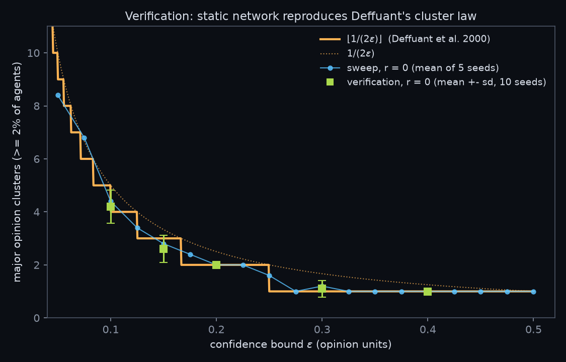
The rule is a rough law, and our counts sit on or just under it at small ε. Two effects push the count down. On a sparse network, agents whose neighbours are all out of range become frozen stragglers, and they are not counted because they fall below the 2% "major" threshold. Neighbouring proto-clusters can also merge before they separate. At ε = 0.30, one seed in ten kept a straggler group of ≥ 2% of agents, which is why the mean is 1.1. The sweep's r = 0 row (blue line) follows the same staircase from ε = 0.05 to 0.5.
2. Exact invariant. The Deffuant update moves both partners by equal and opposite amounts, so the mean opinion is conserved. Measured drift over the 210-step showcase run: $|\langle x\rangle_T - \langle x\rangle_0| = 0.0$ (asserted < 1e-10).
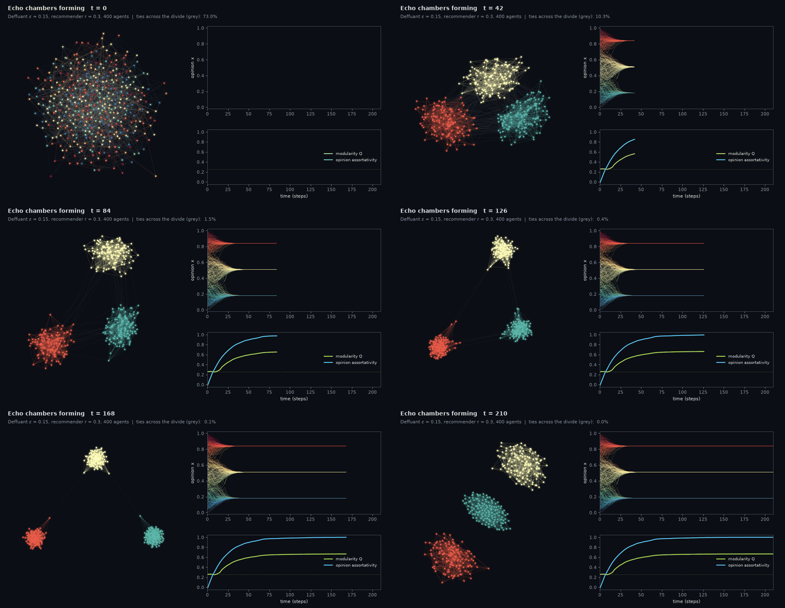
3. Analytic initial condition. For i.i.d. uniform opinions, a tie is "across the divide" ($|\Delta x| \ge \varepsilon$) with probability $1-(2\varepsilon-\varepsilon^2)$ = 72.25% at ε = 0.15. The GIF's first frame measures 73.0% on its 2400 ties.
Phase diagram: ε decides how many camps form, r decides whether they still talk
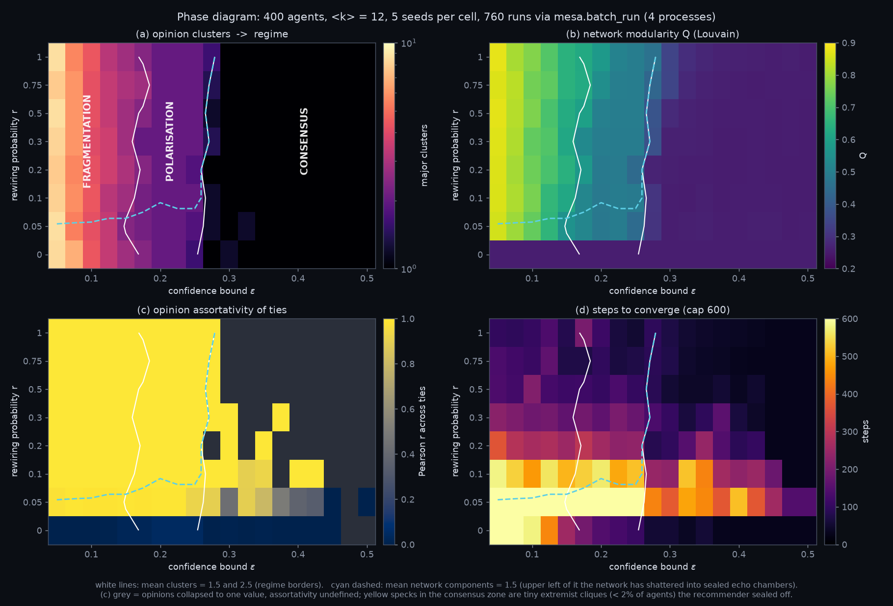
760 runs (19 ε × 8 r × 5 seeds, common random numbers), mesa.batch_run on 4 processes:
| r | consensus for all ε ≥ | Louvain Q at ε = 0.2 | runs where network components = opinion camps |
|---|---|---|---|
| 0 | 0.325 | 0.26 | 54% (only the consensus runs) |
| 0.05 | 0.350 | 0.48 | 52% |
| 0.1 | 0.300 | 0.48 | 87% |
| 0.2 | 0.275 | 0.49 | 100% |
| 0.3 | 0.300 | 0.50 | 100% |
| 0.5 | 0.300 | 0.50 | 100% |
| 0.75 | 0.300 | 0.55 | 100% |
| 1 | 0.300 | 0.58 | 100% |
What the sweep says:
- The number of opinion camps is set by ε, not by the recommender. In panel (a) the regime borders (white lines) are nearly vertical: fragmentation for ε ≲ 0.17, polarisation up to ε ≈ 0.26–0.28, then consensus. Rewiring does not create extra camps.
- The recommender turns camps into sealed echo chambers. With a static network (r = 0), polarised camps stay in one connected network. The cross-camp ties still exist, but they carry no influence because $|\Delta x| > \varepsilon$. Modularity stays at the random-graph baseline Q = 0.26 and opinion assortativity stays ≈ 0 (panel c). For any r ≥ 0.2, the network in 100% of runs shatters into exactly as many connected components as there are opinion camps, with assortativity 1.0. Q climbs to ≈ 0.5 for two camps and close to 0.9 for the 8–9 camps at ε = 0.05 (panel b).
- Even gentle rewiring gets there, just slowly. At r = 0.05 the network has not finished sorting within 600 steps (panel d, runs at the cap). Only 52% of those runs reach "components = camps". Small r means long transients, not a different end state.
- The consensus threshold barely moves (ε ≈ 0.275–0.30 for r ≥ 0.1 vs 0.325 for r = 0, a difference of one or two grid steps). The like-minded recommender even helps near the threshold: it hands stranded agents an in-range partner, where a static network would leave them as stragglers. This differs from Kozma & Barrat (2008), whose rewiring target is random and who report a consensus threshold pushed to larger ε. What the recommender suggests matters.
Trajectories
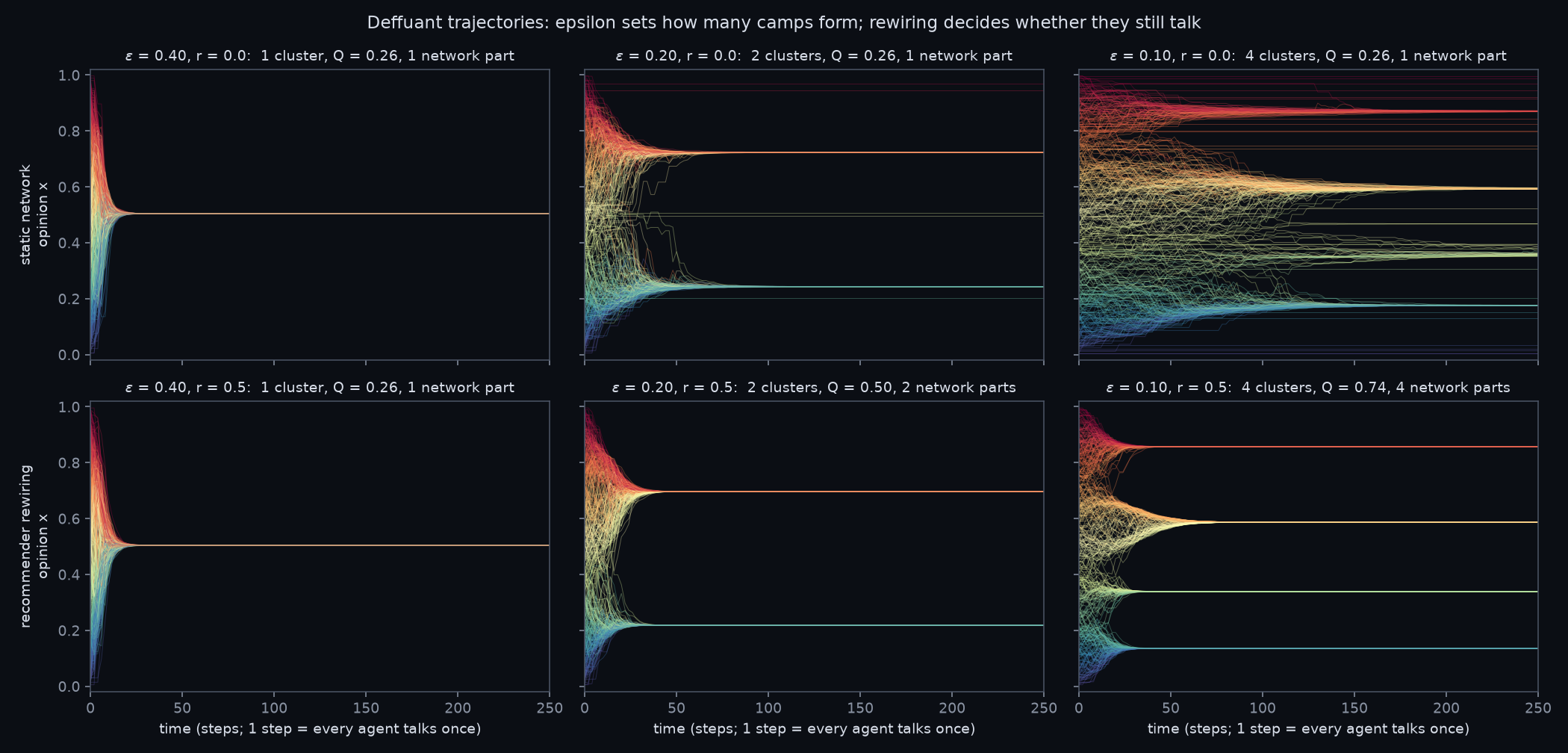
Same seed, same ε, static vs rewiring. At ε = 0.1 both end with 4 clusters, but the static network keeps a halo of frozen stragglers and one connected graph (Q = 0.26). With r = 0.5 the clusters are cleaner and faster, and they sit in 4 separate network components (Q = 0.74). At ε = 0.2 you get 2 clusters in both rows: Q = 0.26 and one component, vs Q = 0.50 and two components.
Showcase run (hero + GIF)
ε = 0.15, r = 0.3, seed 6 (chosen for three similar-sized camps: 136/132/132 agents). It converges in 210 steps to 3 opinion clusters in 3 network components, with Q = 0.67 and opinion assortativity 1.00. The share of ties across the divide falls from 73% to 4.7% by t = 60 and to 0.0% at the end. The GIF (3.4 MB, 71 frames) shows the force-directed layout morph from a hairball into three islands, while the modularity and assortativity curves rise in the corner panel.
Run it
# from SimulationLab/
uv run python L04_echo_chambers/sim.py
Runtime:
- Expected on an idle 8-core machine: about 3 min. This is estimated from stage timings measured when the machine was lightly loaded: verification ≈ 15 s, a comparable 836-run sweep ≈ 50 s on 4 processes, spaghetti ≈ 20 s, showcase + GIF ≈ 60 s.
- Measured while other simulations saturated the CPU (90–100% load): 13.3 min and 19.2 min of in-script time. Stage breakdown of the slower run: verify 248 s, sweep 616 s, spaghetti 93 s, GIF + hero 196 s.
- Nothing uses more than 4 processes.
- Importing Mesa takes ~3 s, and each of the 4 spawned
batch_runworkers pays that cost again.
Stage by stage, the script prints the verification table, a per-r sweep summary, the showcase
statistics, and all checks passed. The assertions fail the run if the cluster law misses by more
than 1 or if the mean opinion drifts.
Outputs in output/: hero.png, echo_chambers.gif, phase_diagram.png, spaghetti.png,
verify_clusters.png.
Code tour (sim.py)
| Piece | What it does |
|---|---|
major_clusters, bimodality, opinion_assortativity |
pure NumPy/SciPy metrics on an opinion vector (and tie list) |
Person(FixedAgent) |
one agent. step() = pick a random neighbour cell, then either Deffuant-average or ask the recommender to rewire |
EchoChamber(mesa.Model) |
builds the G(n,m) graph, wraps it in mesa.discrete_space.Network, creates agents with Person.create_agents, and wires up the DataCollector |
EchoChamber.recommend |
rejection-samples a like-minded stranger (the "recommender") |
EchoChamber.modularity |
Louvain $Q$, cached until the tie structure changes |
EchoChamber.converged / step |
agents.shuffle_do("step"), the convergence test, and data collection at the end (or every collect_every steps) |
verify() |
batch_run at $r = 0$ over 5 ε values × 10 seeds, compared with $\lfloor 1/(2\varepsilon)\rfloor$ |
sweep() |
batch_run over ε × r × seeds on 4 processes, collected into arrays [r, ε, seed] |
run_tracked() |
one run with agent data every every steps (agent_reporters={"opinion": "x"}) and edge-list snapshots |
layouts, draw_network, animate, plot_* |
force-directed layout continued frame to frame, glowing network rendering, and the figures |
main() |
verify → sweep → figures → spaghetti → showcase GIF + hero → assertions |
Simplifications & ceilings
- One-dimensional opinion. Real attitudes are multi-dimensional and issue-bundled. Upgrade: vector opinions with a Euclidean or issue-wise confidence bound.
- Only attraction, never repulsion. Deffuant agents never move away from each other, so this model cannot produce "backfire" polarisation. Upgrade: Jager & Amblard (2005) assimilation/contrast.
- Homogeneous ε. Everyone is equally open-minded. Heterogeneous ε with a few closed-minded extremists changes the outcome drastically (Deffuant et al. 2002).
- Global recommender by rejection sampling (
# ponytail:in the code). It fails silently when like-minded strangers are rare (< ~5% of the population). Upgrade: keep a sorted opinion index and sample from it, or recommend friends-of-friends (triadic closure), which is closer to how real platforms work. - Random-graph start. Real social networks have heavy-tailed degrees, clustering and community
structure before anyone rewires. Upgrade:
nx.powerlaw_cluster_graphor an empirical edge list. - N = 400 and ⟨k⟩ = 12, sized for a ≤ 5-minute run on 4 cores. Louvain in pure Python is the most expensive reporter. Upgrade: igraph/Leiden, or a Numba kernel for the agent loop.
- No noise. With no opinion noise, clusters are absorbing states. Adding noise gives drift and merging on long time scales (Pineda, Toral & Hernández-García 2009).
- Cluster detection by a fixed gap (0.02) and a 2% size threshold. Minor clusters and stragglers are deliberately not counted, as in Deffuant's "major clusters".
Go further
- Rebuild it in NetLogo with BehaviorSpace and check that you reproduce the same phase diagram. This is the standard cross-validation ("docking") exercise from Axtell et al. (1996).
- Friend-of-friend recommender: replace
recommendwith triadic closure. Does it still seal chambers, or does clustering keep bridges alive? - Contrarians and zealots: add agents with $\mu = 0$ (stubborn) or repulsive influence and map where they break consensus.
- Sensitivity analysis: treat $(\varepsilon, r, \mu, \langle k \rangle)$ as uncertain inputs and compute Sobol indices with SALib. That tool arrives in L07.
- Scale up: port the agent loop to Numba or Agents.jl and push to $N = 10^5$. Check whether the consensus threshold sharpens (finite-size scaling, as in L01).
References
- Deffuant, G., Neau, D., Amblard, F. & Weisbuch, G. (2000). Mixing beliefs among interacting agents. Advances in Complex Systems 3, 87–98.
- Weisbuch, G., Deffuant, G., Amblard, F. & Nadal, J.-P. (2002). Meet, discuss, and segregate! Complexity 7(3), 55–63.
- Hegselmann, R. & Krause, U. (2002). Opinion dynamics and bounded confidence: models, analysis and simulation. JASSS 5(3).
- Lorenz, J. (2007). Continuous opinion dynamics under bounded confidence: a survey. Int. J. Mod. Phys. C 18(12), 1819–1838.
- Kozma, B. & Barrat, A. (2008). Consensus formation on adaptive networks. Phys. Rev. E 77, 016102.
- Holme, P. & Newman, M. E. J. (2006). Nonequilibrium phase transition in the coevolution of networks and opinions. Phys. Rev. E 74, 056108.
- Gross, T. & Blasius, B. (2008). Adaptive coevolutionary networks: a review. J. R. Soc. Interface 5, 259–271.
- Sasahara, K., Chen, W., Peng, H., Ciampaglia, G. L., Flammini, A. & Menczer, F. (2021). Social influence and unfollowing accelerate the emergence of echo chambers. J. Computational Social Science 4, 381–402.
- Castellano, C., Fortunato, S. & Loreto, V. (2009). Statistical physics of social dynamics. Rev. Mod. Phys. 81, 591.
- Flache, A. et al. (2017). Models of social influence: towards the next frontiers. JASSS 20(4), 2.
- Jager, W. & Amblard, F. (2005). Uniformity, bipolarization and pluriformity captured as generic stylized behavior with an agent-based simulation model of attitude change. Comput. Math. Organ. Theory 10, 295–303.
- Grimm, V. et al. (2006). A standard protocol for describing individual-based and agent-based models. Ecological Modelling 198, 115–126. Updated: Grimm, V. et al. (2020). The ODD protocol for describing agent-based and other simulation models: a second update. JASSS 23(2), 7.
- Blondel, V. D., Guillaume, J.-L., Lambiotte, R. & Lefebvre, E. (2008). Fast unfolding of communities in large networks. J. Stat. Mech. P10008 (Louvain).
- Newman, M. E. J. (2003). Mixing patterns in networks. Phys. Rev. E 67, 026126 (assortativity).
- Pfister, R. et al. (2013). Good things peak in pairs: a note on the bimodality coefficient. Frontiers in Psychology 4, 700.
- Axtell, R., Axelrod, R., Epstein, J. M. & Cohen, M. D. (1996). Aligning simulation models: a case study and results. Comput. Math. Organ. Theory 1, 123–141.
- ter Hoeven, E. et al. (2025). Mesa 3: Agent-based modeling with Python in 2025. Journal of Open Source Software.
- Railsback, S. F. & Grimm, V. (2019). Agent-Based and Individual-Based Modeling: A Practical Introduction, 2nd ed. Princeton UP.
- Wilensky, U. & Rand, W. (2015). An Introduction to Agent-Based Modeling. MIT Press.