L03: ATL Checkpoint
How many screening lanes does the world's busiest airport need, hour by hour? A discrete-event simulation of a TSA checkpoint, checked against queueing theory and tuned by simulation optimisation.
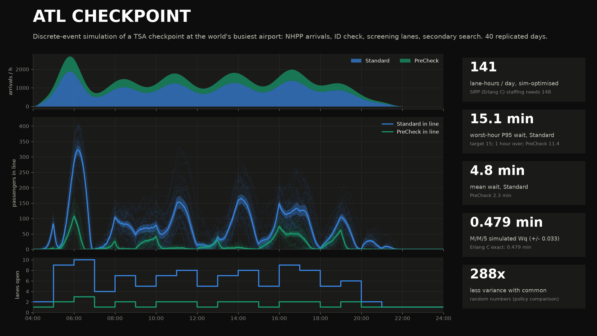
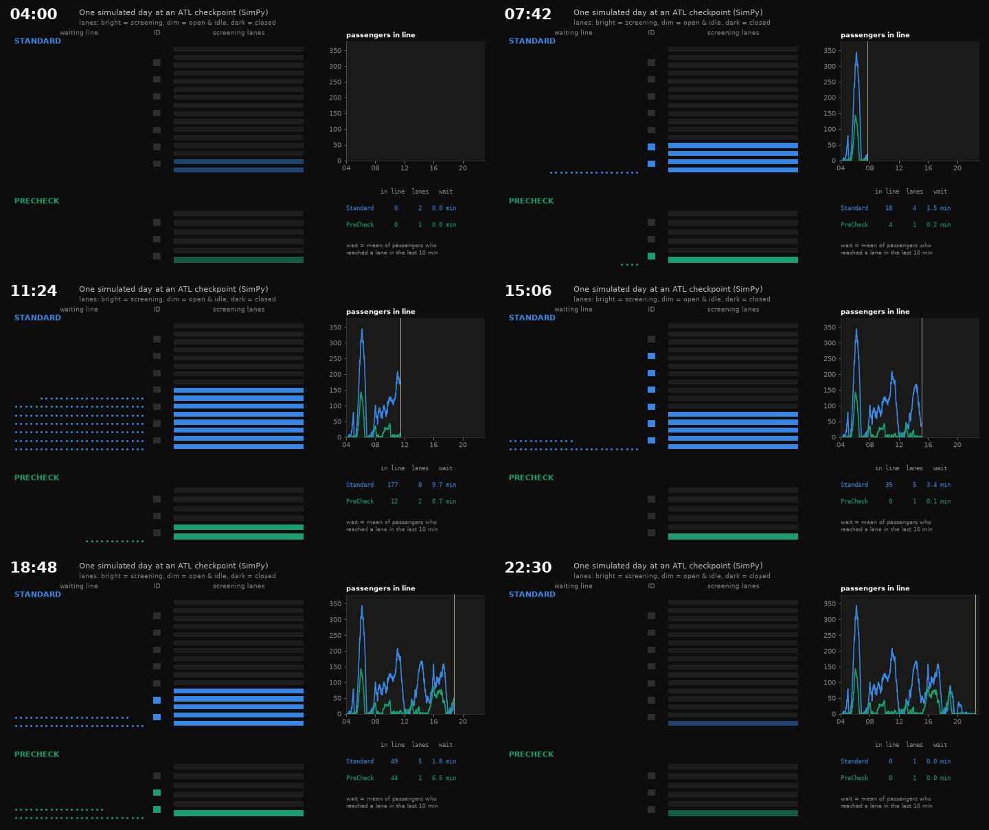
One simulated day at the checkpoint: the serpentine line, ID podiums, and screening lanes opening and closing on the optimised schedule.
1. The question
Hartsfield–Jackson (ATL) handled 108.06 million passengers in 2024 and was again the world's busiest airport (ACI World ranking, ATL press release). TSA screened a record 30.1 million people at ATL in 2025 (about 82,000 per day on average) and 111,624 on its record day (4 April 2025). The 108 million counts arrivals and departures, so roughly 54 million people departed. Only about 30 million of them passed a checkpoint; the rest were connecting passengers, mostly on Delta, who never leave the secure side.
Screening lanes are expensive. Each one needs a team of officers, and TSA plans staffing hour by hour. So the question is:
What is the cheapest hourly lane schedule for one checkpoint such that, in every hour of the day, 95% of passengers wait at most 15 minutes before screening?
A spreadsheet can't answer it well: arrivals come in banks, queues carry over from one hour to the next, and the 95th percentile depends on the whole wait distribution, not the mean. That is what discrete-event simulation (DES) is for.
2. The model
Passenger flow (per stream: Standard and PreCheck, each with its own podiums and lanes).
NHPP arrivals ──► ID/document check (c_TDC podiums) ──► screening lane (n_k(h) open lanes) ──► [prob. q] secondary bag search ──► airside
                      FCFS queue                           FCFS queue, lanes open/close hourly         shared pool of officers
- Arrivals: a non-homogeneous Poisson process with rate λ(t). The daily shape is a sum of six Gaussian "banks" (Delta's hub departure waves, seen 1–2 h earlier at the checkpoint), scaled so that ∫λ(t)dt = 22,000 passengers/day. Arrivals run from 04:00 to 22:00. Each passenger is PreCheck with probability 0.30.
- Random variates: ID check ~ Gamma(k=3, mean 10 s). Lane time per passenger ~ Gamma(k=2, mean 60/μ), where μ = 150/h for a standard lane and 300/h for PreCheck. Secondary search happens with probability q = 0.10 (Standard) or 0.05 (PreCheck) and takes ~ Gamma(k=2, mean 3 min).
- Staffing decision: n_k(h) = open lanes of stream k in hour h, for 20 blocks from 04:00 to 24:00. When a lane closes, it finishes the passenger it is screening first.
- Performance measure: wait = time in queues before screening starts (ID queue + lane queue), which is what TSA's posted wait times measure.
- Constraint: for every hour h and stream k, P(wait > 15 min | arrived in hour h) ≤ 5%, i.e. the hourly P95 ≤ 15 min. Cost = lane-hours per day.
What is anchored to public data and what is assumed. Please read this table before quoting any number from this project.
| Parameter | Value used | Status | Basis |
|---|---|---|---|
| ATL annual passengers | 108.06 M (2024) | public | ACI World / ATL press release, Apr 2025 |
| ATL TSA-screened passengers | 30.1 M in 2025 (~82k/day), record day 111,624 | public | AJC (Jan 2026), Atlanta News First (Apr 2025) |
| Passengers at this checkpoint | 22,000/day | assumption | ATL's ~82k/day are split over several checkpoints. We model one busy one. |
| Standard lane throughput | 150 pax/h | public, order of magnitude | TSA figures quoted in the press: a PreCheck lane screens ~300/h, "twice a standard lane" |
| PreCheck lane throughput | 300 pax/h | public, order of magnitude | same; DHS S&T's "300 people per hour per lane" programme |
| TSA wait-time standards | < 30 min standard, < 10 min PreCheck | public | TSA. Shown for context only; our target is the stricter 15 min per hour |
| Daily arrival shape (banks) | 6 Gaussian bumps, peak 05:00–06:00 | assumption | qualitative hub banking; no public hourly checkpoint data |
| PreCheck share | 30% | assumption | |
| ID check time, lane-time CV | 10 s (CV 0.58), CV 0.71 | assumption | |
| Podiums / physical lanes | 7 + 3 / 16 + 6 | assumption | |
| Secondary search | q = 10% / 5%, 3 min, 12 officers | assumption | only affects time in system, not the wait |
So the structure and the method are realistic, and the scale is plausible, but the lane counts below are not a recommendation for the real ATL checkpoints. Treat them as the output of a well-verified model with made-up inputs where the table says "assumption".
3. M&S concepts you'll learn here
- Two DES worldviews. Event scheduling: a future-event list (a heap) plus one routine per event type (
mmc_events). Process interaction: write the life of one entity as a generator and let the library own the event list (SimPy,mmc_simpy,run_day). Given the same inputs they produce bit-identical waits. - Random variate generation: NHPP by thinning (Lewis & Shedler 1979). Generate candidates at a constant λ_max and keep a candidate at time t with probability λ(t)/λ_max.
- Terminating vs steady-state simulation. The checkpoint day is terminating: it starts empty at 04:00, and that is the real initial condition, so there is no warm-up to delete. The M/M/c verification model is steady-state, so its start-up bias must be removed.
- Initialisation bias and Welch's procedure. Ensemble-average the i-th customer's wait across replications, smooth it, and see where it flattens.
- Output analysis. Independent replications, t-based confidence intervals, and a coverage experiment that tests whether "95%" CIs really cover 95% of the time.
- Verification against queueing theory. Erlang C gives Wq and the full tail P(Wq > t) of M/M/c.
- Common random numbers (CRN). Pre-generate all of a day's randomness per seed, so every policy sees the same passengers. Paired differences then have far lower variance.
- Simulation optimisation. An analytic starting point (SIPP: stationary independent period-by-period Erlang C), then a greedy search scored by simulation.
- Optimisation bias (the "optimiser's curse"). A plan tuned to pass on a few replications fails on fresh ones. The fix is more replications and a statistical feasibility test (an upper confidence bound).
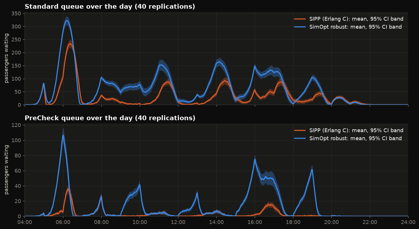
- Time-varying queues. Peaks and lags mean a queue built at 06:00 is still there at 06:40. This is why hour-by-hour steady-state formulas misjudge staffing in both directions.
4. Tech stack
| Tool | Role here | Why it matters |
|---|---|---|
| Python 3.12 | everything | |
| NumPy | variate generation, CRN day tapes, output statistics | vectorised pre-generation keeps random streams synchronised |
| Matplotlib | figures + GIF (PillowWriter) | |
| SciPy | scipy.stats.t quantiles for CIs |
|
| ★ SimPy 4 | process-interaction DES engine: Environment, Resource, generators as processes |
the Python counterpart of Arena/SIMAN process blocks. It is free and scriptable, so optimisation loops are easy |
★ heapq + collections.deque |
hand-written event-scheduling engine | shows what every DES engine does inside, and runs 10-15x faster than SimPy for a single queue |
★ multiprocessing.Pool(4) |
replications in parallel | replications are embarrassingly parallel |
| ★ Queueing theory (Erlang B/C) | yardstick and starting solution | the analytic model you verify against and the heuristic you try to beat |
5. Industry & scientific tools
| Tool | What it is | Typically used for / by | How this project maps to it |
|---|---|---|---|
| Arena (Rockwell) | Flowchart DES on the SIMAN language. Create → Process → Decide → Dispose modules, plus OptQuest and Input/Output Analyzers | The classic teaching tool (ISyE courses use it). Manufacturing, healthcare, call centres, government | run_day = Create (NHPP schedule) → Seize-Delay-Release (ID, lane) → Decide (q) → Process. Lane schedules = Arena Schedules on a Resource. OptQuest ≈ our optimise |
| Simio | Object-oriented DES with 3D animation, built by the Arena authors (Pegden). Risk-based planning and scheduling | Manufacturing digital twins, airports, hospitals, supply chains | Checkpoint = Source → Servers with work schedules → Sink. Simio's experiments with replications, CRN and the OptQuest/KN add-ins map to sections 6.3–6.5 |
| AnyLogic | Multi-method platform in Java: DES (Process Modeling Library), agent-based, system dynamics, and a Pedestrian Library | Airports and terminals (passenger flow in 2D/3D space), logistics, rail, business strategy | Our queues are abstract. AnyLogic would model the serpentine as physical space with walking pedestrians. Its optimisation experiment uses OptQuest |
| FlexSim | 3D object-based DES with realistic visuals, plus FlexSim HC for healthcare | Warehousing, material handling, manufacturing lines, healthcare | Lanes = Processors, podiums = Queues + Processors, and the hourly staffing = Time Tables |
| SimPy / salabim | Open-source Python process-interaction DES. salabim adds built-in animation and monitors | Research, teaching, custom tools that need Python's ecosystem (optimisers, ML, pandas) | This project. salabim would give the animated checkpoint almost for free |
| CAST Terminal (ARC), AirTOP | Specialised airport-terminal simulators | Airport planners and consultancies sizing checkpoints, check-in and gates | The domain-specific version of what is built here from scratch |
| Erlang calculators / queueing theory | Closed-form M/M/c (Erlang C), Erlang A, square-root staffing | Call-centre workforce management (NICE, Verint), first-cut TSA/airport sizing | sipp_plan() is exactly this, and section 6.4 shows where it is wrong |
6. Results
All numbers below come from the default run (python L03_atl_checkpoint/sim.py, fixed seeds).
6.1 Random variates: NHPP thinning
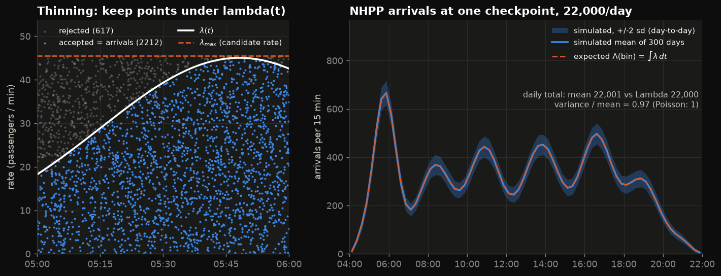
On the left, one hour of candidates: a candidate is kept if it falls under λ(t). Near the 05:50 peak almost all are kept, and at 05:00 about 60% are rejected. On the right are 300 simulated days. Mean daily count 22,001.3 vs Λ = 22,000.0 (z = +0.15), variance/mean = 0.967 (Poisson predicts 1).
6.2 Verification: two worldviews vs Erlang C
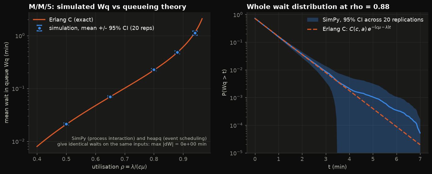
M/M/5 with λ = 11/min and μ = 2.5/min (5 lanes at 150/h, ρ = 0.88), 20 replications × 22,000 customers, deleting the first 2,000:
| Check | Theory | Simulation | Result |
|---|---|---|---|
| SimPy vs heapq event list, same 22,000 inputs | identical | max |ΔW| = 0.0 min | exact |
| Wq at ρ = 0.88 (SimPy) | 0.4789 min | 0.4793 ± 0.0329 | inside 95% CI ✔ |
| P(wait > 0) | 0.7184 | 0.7234 ± 0.0090 | inside ✔ |
| Wq, ρ = 0.50 / 0.65 / 0.80 / 0.94 | 0.0209 / 0.0692 / 0.2216 / 1.1389 | 0.0211±0.0009 / 0.0699±0.0022 / 0.2265±0.0112 / 1.1227±0.0956 | all inside ✔ |
The right panel checks the whole distribution, P(Wq > t) = C(c,a)·e^{−(cμ−λ)t}. The band is a 95% CI across replications. It widens in the far tail because waits are strongly autocorrelated: one long busy period produces hundreds of long waits in a row.
In the logged run, SimPy took 0.87 s and the heapq engine 0.058 s for the same 22,000 customers, so the hand-written engine was about 15× faster. The library buys readability and composability, not speed.
6.3 Warm-up and why it matters: Welch + CI coverage
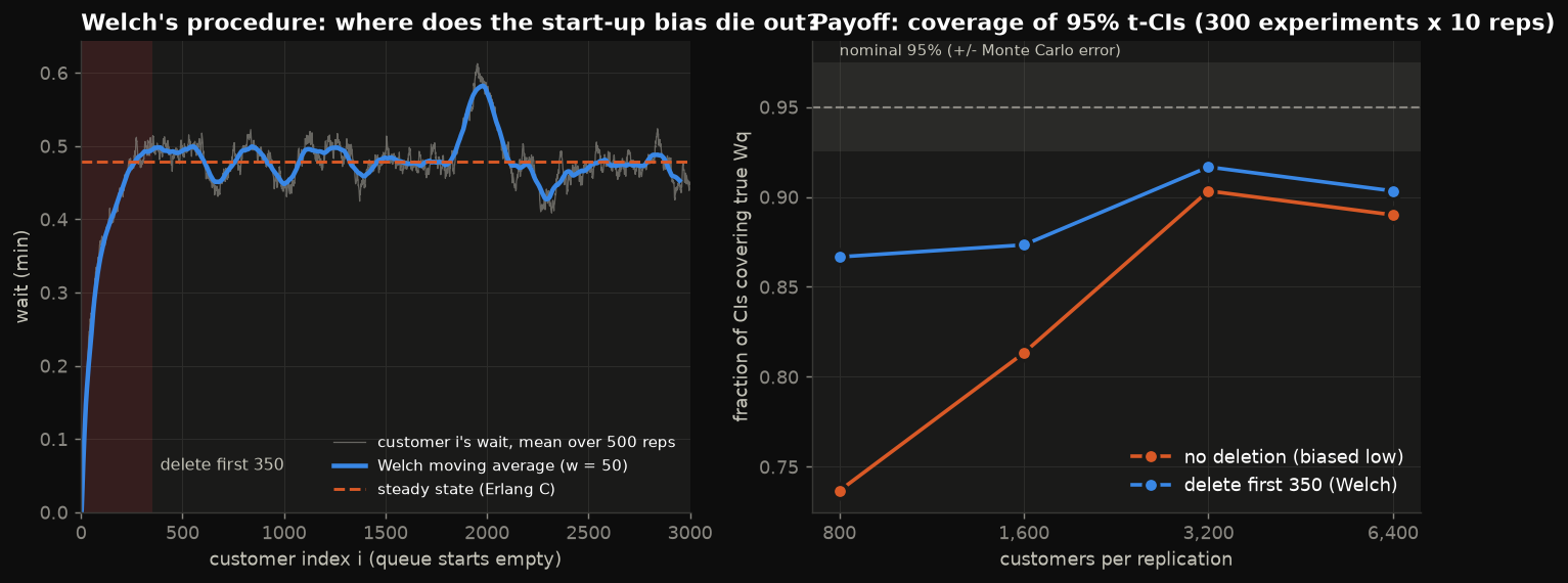
Starting M/M/5 empty and averaging 500 replications, Welch's moving average first reaches 95% of its plateau after roughly 230 customers. We delete d = 350 (1.5× safety, rounded up to 50). The coverage experiment then builds 300 independent "95%" confidence intervals (10 replications each) and counts how many contain the true Erlang-C Wq (Monte Carlo error about ±0.025):
| customers per replication | no deletion | delete first 350 |
|---|---|---|
| 800 | 0.737 | 0.867 |
| 1,600 | 0.813 | 0.873 |
| 3,200 | 0.903 | 0.917 |
| 6,400 | 0.890 | 0.903 |
Deleting the warm-up clearly helps. Even with deletion, coverage stays below 95%. With ρ = 0.88, replication means are right-skewed (rare long busy periods), and a t-interval from 10 replications assumes normality. Longer runs or more replications fix it slowly. This is a real, commonly underestimated effect in heavy-traffic simulation, not a bug.
6.4 Staffing: SIPP vs simulation optimisation
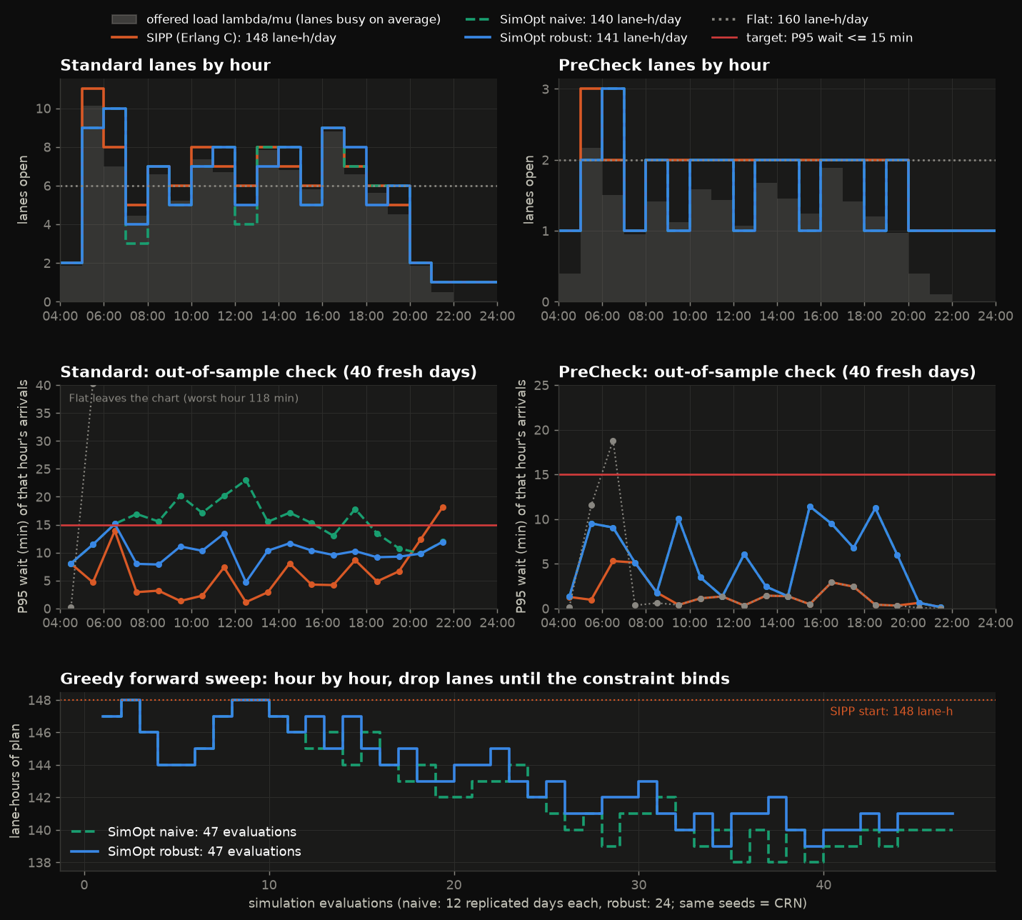
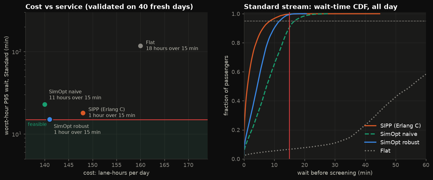
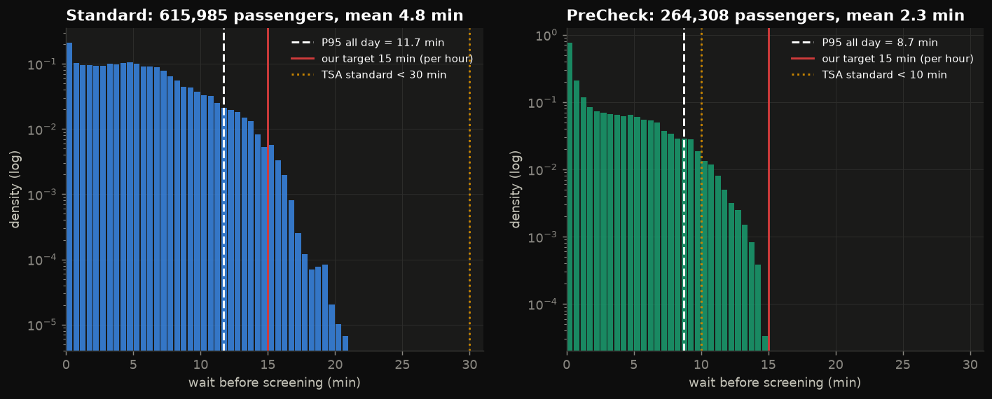
Four policies, all validated on 40 fresh replications that were never used to design them (waits in minutes):
| policy | lane-h/day | mean wait std / pre (± 95% CI) | day P95 std / pre | worst-hour P95 std / pre | hours with P95 > 15 (std/pre) | worst hour: P(wait > 15), std |
|---|---|---|---|---|---|---|
| SIPP (Erlang C per hour) | 148 | 2.29 ± 0.17 / 0.48 ± 0.03 | 8.71 / 2.39 | 18.14 / 5.30 | 1 / 0 | 6.2% ± 7.1% (21:00) |
| SimOpt naive (12 reps, point estimate) | 140 | 7.85 ± 0.79 / 2.34 ± 0.13 | 15.23 / 8.39 | 22.98 / 11.43 | 11 / 0 | 34.4% ± 12.7% (09:00) |
| SimOpt robust (24 reps, upper conf. bound) | 141 | 4.78 ± 0.31 / 2.34 ± 0.13 | 11.48 / 8.39 | 15.13 / 11.43 | 1 / 0 | 5.8% ± 4.3% (06:00) |
| Flat (same lanes all day, 6 + 2) | 160 | 58.04 ± 1.67 / 1.34 ± 0.11 | 102.5 / 10.53 | 117.7 / 18.80 | 17 / 1 | 100% (06:00) |
Lane schedules found (standard lanes, 04:00 → 23:00):
SIPP (Erlang C)  [2, 11, 8, 5, 7, 6, 8, 7, 6, 8, 7, 6, 9, 7, 6, 5, 2, 1, 1, 1]
SimOpt naive     [2,  9, 10, 3, 7, 5, 7, 8, 4, 8, 8, 5, 9, 7, 6, 6, 2, 1, 1, 1]
SimOpt robust    [2,  9, 10, 4, 7, 5, 7, 8, 5, 7, 8, 5, 9, 8, 5, 6, 2, 1, 1, 1]
PreCheck (both SimOpt runs) [1, 2, 3, 1, 2, 1, 2, 2, 1, 2, 2, 1, 2, 2, 1, 2, 1, 1, 1, 1]  (SIPP: 35 lane-h, SimOpt: 31)
What to take from it:
- SIPP overstaffs and understaffs at the same time. Each hour is treated as a steady-state M/M/c at that hour's average rate. With a 15-minute target and 24-second services, that just means "keep ρ < 1", so SIPP spends 148 lane-hours. It still misses at 21:00, because it drops to one lane while the 20:00 backlog is still in the queue.
- Queues are a buffer you can spend, and lags are a debt you must pay. The optimised plan runs below the offered load λ/μ at the start of a bank (05:00: 9 lanes for a load of 10.1; also 07:00, 09:00, 15:00, 18:00) and lets the line absorb it. It then runs above the load in the next hour (06:00: 10 lanes for a load of 7.0) to clear the backlog. This is the classic lag effect of time-varying queues that SIPP cannot see. Net saving: 7 lane-hours a day (−4.7%) compared with SIPP.
- The optimiser's curse is real. The naive search passed every hour on its own 12 replications but fails 11 hours on fresh days, and its worst hour has 34% of passengers waiting more than 15 min. It overfitted lucky sample paths: the day-to-day sd of an hourly P95 is 2–6 min. Requiring the upper 95% confidence bound of P(wait > 15) to be ≤ 5% on 24 replications costs one extra lane-hour and removes almost all of it.
- Honest miss: the robust plan's worst hour (06:00) validates at P95 = 15.13 min, and P(wait > 15) = 5.8% ± 4.3%. That is on the boundary, and the CI comfortably contains 5%, so it is within the validation's own sampling error. A stricter bound (z = 1.64) or more replications would buy margin.
- Timing beats volume. Flat staffing with more lane-hours (160) is a disaster at the 06:00 bank.
Time in system (including secondary bag search) under the robust plan: 5.65 ± 0.31 min for Standard and 2.86 ± 0.13 min for PreCheck.
6.5 Common random numbers
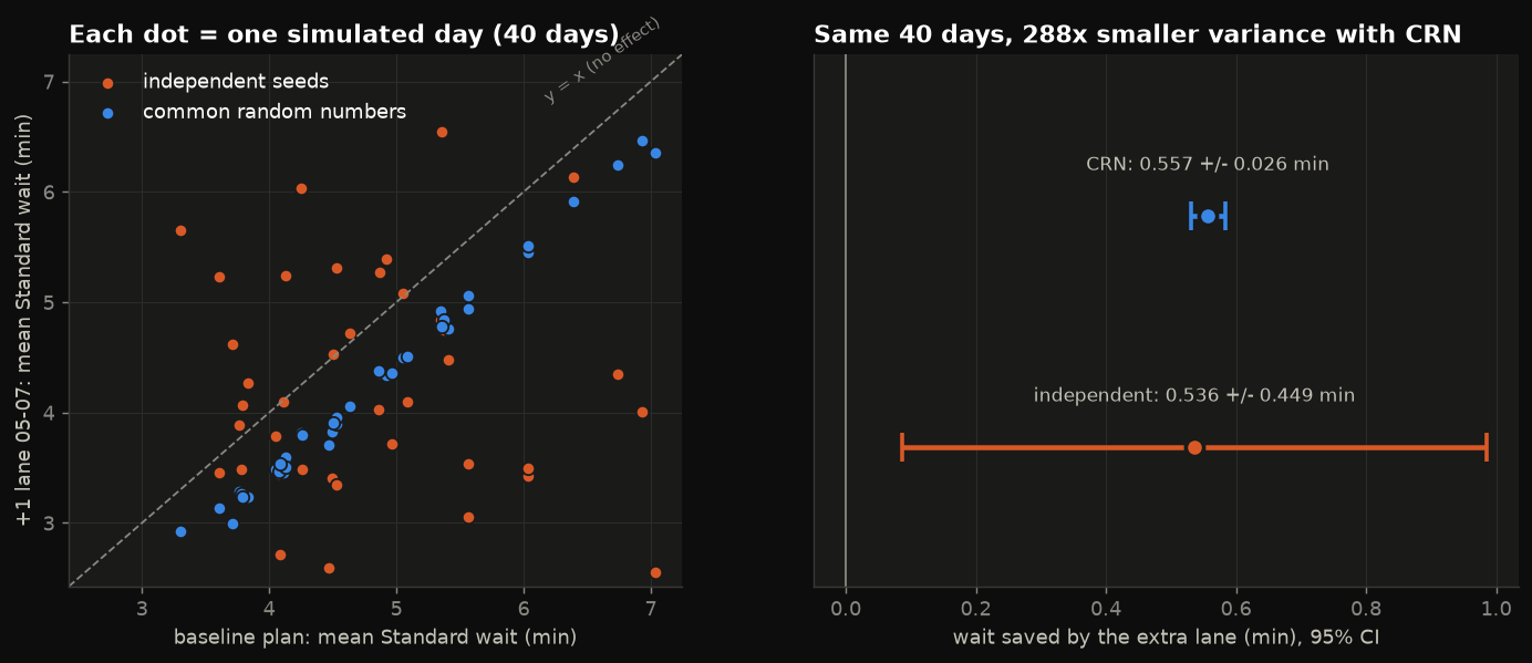
Question: how much does one extra standard lane from 05:00 to 07:00 cut the average standard wait?
| sampling | estimated saving (min) | 95% CI half-width |
|---|---|---|
| independent seeds | 0.536 | ± 0.449 |
| CRN (same 40 days) | 0.557 | ± 0.026 |
The variance of the paired difference drops by 288× (correlation 0.996). To match CRN's precision with independent sampling you would need about 288 times as many replicated days.
7. Run it
# from SimulationLab/
uv run python L03_atl_checkpoint/sim.py
Output: printed verification + policy tables, and output/*.png, output/checkpoint.gif.
Runtime: the logged run below took 232 s (3.9 min) with 4 worker processes on the shared 8-core machine, with other agents' jobs running at the same time. The two sim-optimisation sweeps (47 evaluations × 12 or 24 replicated days) take about 60% of it, followed by the GIF, the 160-day validation and the CRN runs. Under heavy contention (another process holding about 8 threads) an identical run took 31 min. To make it faster, drop the naive sweep or cut the robust seeds from 24 to 16 in main().
Console output of the logged run
=== VERIFICATION ===
[1] SimPy vs event scheduling, same 22000 inputs: max |dW| = 0.0e+00 min (SimPy 0.87 s, heapq 0.058 s)
[2] M/M/5 rho=0.88: Erlang-C Wq = 0.4789 min, SimPy 20 reps = 0.4793 +/- 0.0329
    P(wait>0): Erlang-C 0.7184, sim 0.7234 +/- 0.0090
    rho=0.50: Wq theory 0.0209, sim 0.0211 +/- 0.0009  ok
    rho=0.65: Wq theory 0.0692, sim 0.0699 +/- 0.0022  ok
    rho=0.80: Wq theory 0.2216, sim 0.2265 +/- 0.0112  ok
    rho=0.88: Wq theory 0.4789, sim 0.4851 +/- 0.0289  ok
    rho=0.94: Wq theory 1.1389, sim 1.1227 +/- 0.0956  ok
[3] NHPP thinning, 300 days: daily count mean 22001.3 vs Lambda 22000.0 (z=+0.15), var/mean = 0.967 (Poisson: 1)
[4] Welch warm-up d = 350 customers. 95% CI coverage over 300 macro-reps (nominal 0.95):
    run length   800: no deletion 0.737, delete first 350: 0.867
    run length  1600: no deletion 0.813, delete first 350: 0.873
    run length  3200: no deletion 0.903, delete first 350: 0.917
    run length  6400: no deletion 0.890, delete first 350: 0.903

=== STAFFING POLICIES (validated on 40 fresh seeds; waits in min) ===
policy           lane-h   mean wait std / pre      day P95 std / pre   worst-hour P95 std / pre  hours>15   worst-hour P(wait>15) std
SIPP (Erlang C)    148     2.29+/-0.17 /  0.48+/-0.03     8.71 /  2.39       18.14 /   5.30         1/0        6.2% +/- 7.1% (21:00)
SimOpt naive       140     7.85+/-0.79 /  2.34+/-0.13    15.23 /  8.39       22.98 /  11.43         11/0       34.4% +/- 12.7% (09:00)
SimOpt robust      141     4.78+/-0.31 /  2.34+/-0.13    11.48 /  8.39       15.13 /  11.43         1/0        5.8% +/- 4.3% (06:00)
Flat               160    58.04+/-1.67 /  1.34+/-0.11   102.52 / 10.53      117.71 /  18.80         17/1      100.0% +/- 0.0% (06:00)

CRN: +1 standard lane 05-07 cuts mean standard wait by 0.557 +/- 0.026 min (CRN) vs 0.536 +/- 0.449 (independent); variance ratio 288x, corr 0.9963
8. Code tour
| File / function | What it does |
|---|---|
sim.py top |
All parameters, each tagged (P) public or (A) assumption |
rate, nhpp_thinning |
λ(t) and Lewis–Shedler thinning |
make_day(seed) |
Pre-generates one day's passengers and all their service times, so CRN are synchronised by construction |
run_day(day, plan) |
The SimPy model: passenger process (ID → lane → secondary), source, lane_controller (hourly capacity) |
erlang_c, mmc_wq, mmc_p_wait_gt |
Queueing-theory yardstick (stable Erlang-B recursion) |
mmc_simpy / mmc_events |
Same M/M/c in the two worldviews |
t_ci, welch_ma, _coverage_task |
Output analysis: CIs, Welch smoothing, coverage experiment |
exceed, hourly_p95, summarize |
Service-level statistics per hour and stream |
sipp_plan |
Analytic starting schedule (Erlang C, hour by hour) |
optimise(start, seeds, z) |
Greedy forward sweep. z = 0 is naive, z = 1 is the upper-confidence-bound test |
exp_*, verify, main |
Experiments, assertions, orchestration (Pool of 4) |
plots.py |
All figures, the hero and the animated checkpoint |
9. Simplifications & ceilings
- Unlimited buffer between ID check and lanes. Real checkpoints are space-limited, so the lane queue backs up into the ID queue (blocking). Total wait is barely affected because the lanes are the bottleneck. The animation draws everyone as one line.
- A lane is a single server with service rate = lane throughput. Physically a lane is a pipeline (divest, X-ray, body scanner, re-compose) that serves several people at once. Only the throughput and variability matter for the queue, but lane-level effects are lost, such as bins, CT scanners, and alarms that stop the belt.
- Hourly staffing with instant opening. No shift-length or break constraints, and no officer cross-training between PreCheck and standard. A real TSA roster is a set-covering problem over shifts (see "Go further").
- Greedy optimiser (
# ponytail:in code). It is not a proven optimum. The search is myopic hour by hour, so an early extra lane that saves two later ones would be missed. - Arrivals are exogenous. Passengers don't arrive earlier when lines are long, don't switch streams, and don't miss flights. The daily volume is Poisson with no day-to-day demand shocks (weather, holidays), so real variability is larger.
- No real hourly data. TSA publishes airport-level daily throughput but not per-checkpoint hourly counts, so the arrival shape is an assumption.
- Secondary search uses a shared officer pool and doesn't block lanes.
- Changing lane capacity uses SimPy's private
Resource._capacity. The documented idiom (aPriorityResourceplus high-priority "lane closed" tokens) gave bit-identical results in testing but was about 1.7× slower, because SimPy re-sorts a priority queue on every request. If a future SimPy release breaks this, switch back to the token version.
10. Go further
- Rebuild it in Arena or Simio. Create module with an arrival Schedule, Process modules with Resource Schedules, then OptQuest over the lane counts. Compare your Wq and P95 with these numbers using the same parameter table. Then do the same in AnyLogic with the Pedestrian Library to see how physical space changes the line.
- Shift scheduling. Turn hourly lane requirements into 8-hour shifts with breaks (set-covering integer program with
scipy.optimize.milp), then simulate the roster to check it still meets the target. - Ranking & selection. Replace the greedy feasibility check with a proper procedure: Kim–Nelson KN for the best of k plans, or a stochastically constrained R&S procedure (Andradóttir & Kim) for "cheapest feasible".
- Real data. Scrape the MyTSA wait-time API or TSA's FOIA throughput files (hourly by checkpoint for some airports) to fit λ(t). Then validate the model against observed waits instead of assuming.
- Better time-varying staffing theory. Implement the lagged / pointwise-stationary fluid approximation (Green, Kolesar & Whitt 2007) or the modified-offered-load (MOL) method, and see how close analytic staffing gets to the simulation optimum.
11. References
- A. M. Law, Simulation Modeling and Analysis, 5th ed., McGraw-Hill, 2015. Output analysis, Welch, CRN.
- J. Banks, J. S. Carson, B. L. Nelson, D. M. Nicol, Discrete-Event System Simulation, 5th ed., Pearson, 2010. Worldviews, event scheduling vs process interaction.
- B. L. Nelson, Foundations and Methods of Stochastic Simulation, 2nd ed., Springer, 2021.
- P. A. W. Lewis, G. S. Shedler, "Simulation of nonhomogeneous Poisson processes by thinning," Naval Research Logistics Quarterly 26(3), 1979.
- P. D. Welch, "The statistical analysis of simulation results," in The Computer Performance Modeling Handbook, 1983.
- L. V. Green, P. J. Kolesar, J. Soares, "Improving the SIPP approach for staffing service systems that have cyclic demands," Operations Research 49(4), 2001.
- L. V. Green, P. J. Kolesar, W. Whitt, "Coping with time-varying demand when setting staffing requirements for a service system," Production and Operations Management 16(1), 2007.
- M. Defraeye, I. Van Nieuwenhuyse, "Staffing and scheduling under nonstationary demand for service: A literature review," Omega 58, 2016.
- S.-H. Kim, B. L. Nelson, "A fully sequential procedure for indifference-zone selection in simulation," ACM TOMACS 11(3), 2001.
- M. C. Fu (ed.), Handbook of Simulation Optimization, Springer, 2015.
- D. Gross, J. F. Shortle, J. M. Thompson, C. M. Harris, Fundamentals of Queueing Theory, 4th ed., Wiley, 2008. Erlang C.
- SimPy documentation, https://simpy.readthedocs.io
- Data anchors: ATL press release on ACI 2024 rankings (atl.com, Apr 2025). AJC, "Atlanta hit TSA record in 2025 with 30 million passengers" (Jan 2026). Atlanta News First, ATL screening record 111,624 (Apr 2025). DHS S&T, "300 People Per Hour Per Lane". Fox News / AP, "A long wait: Fliers brace for big security lines at airports" (PreCheck ~300/h, twice a standard lane). TSA wait-time standards (TSA / House hearing "Assessing the TSA Checkpoint", 2017).