L06 · Virtual Wind Tunnel
A lattice Boltzmann CFD solver in one Python file, compiled by Numba, taken through the same verification & validation workflow that professional CFD teams use. First prove the code solves its equations right, then prove they are the right equations, and only then fly a wing through it.
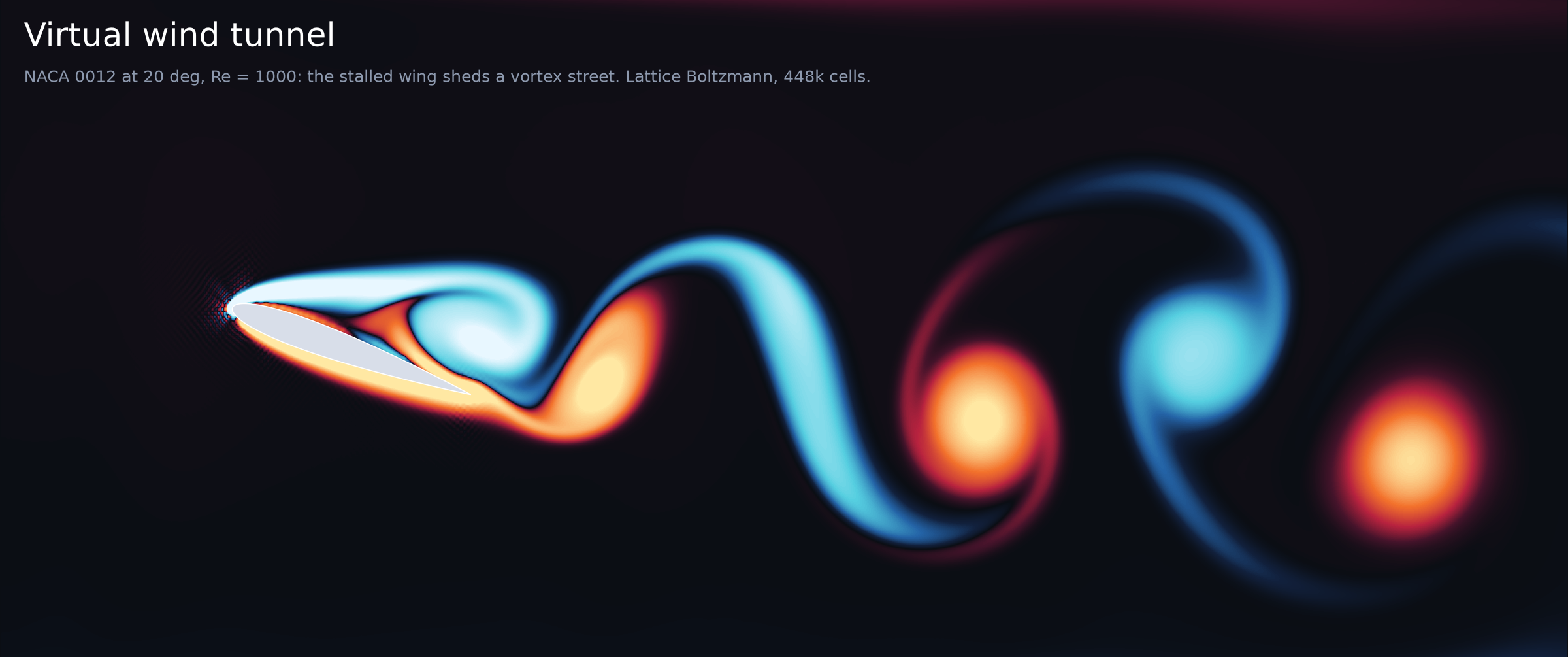
Movie: output/wind_tunnel.mp4 (1280×720, 16 s, H.264). NACA 0012 at 20°,
Re = 1000, chord 128 cells, 448 000 lattice nodes. Colour is vorticity ω c/U: blue is clockwise, orange is
counter-clockwise, and still air is dark. The strip below shows the live lift and drag coefficients.
1. The question
A CFD code will always produce a colourful picture. The hard question is whether you can believe the numbers. This level builds a small but real wind tunnel and asks, in order:
- Verification. Does the solver reproduce an exact solution of the Navier–Stokes equations, and does its error shrink at the rate theory predicts?
- Solution verification. On a real problem with no exact answer (a cylinder in a channel), how big is the discretisation error, and does it converge to the international benchmark?
- Validation. Does a cylinder in free stream shed vortices at the frequency measured in real experiments (Williamson 1996)? Which of our modelling choices (grid, Mach number, tunnel walls, inlet) cause which part of the disagreement?
- Showcase. What does a NACA 0012 wing do at Re = 1000 (the insect / micro-drone regime) from 0° to 20°? Lift curve, drag polar, stall and vortex shedding.
- Limits. Why can't a laptop LBM fly an airliner wing at Re = 10⁷, and what do industrial codes do instead?
2. The model
Lattice Boltzmann instead of Navier–Stokes. LBM does not discretise the Navier–Stokes equations directly. It evolves particle distribution functions $f_i(\mathbf x,t)$: the density of fictitious particles moving with one of nine lattice velocities $\mathbf c_i$ (D2Q9: rest, 4 axis neighbours, 4 diagonals). One time step is two operations:
$$\underbrace{f_i(\mathbf x+\mathbf c_i,\,t+1)}_{\text{stream}} = \underbrace{f_i + \omega\,\big(f_i^{eq}-f_i\big)}_{\text{collide (BGK)}},\qquad f_i^{eq}=w_i\,\rho\Big(1+3\,\mathbf c_i\!\cdot\!\mathbf u+\tfrac92(\mathbf c_i\!\cdot\!\mathbf u)^2-\tfrac32 u^2\Big)$$
with $\rho=\sum_i f_i$, $\rho\mathbf u=\sum_i \mathbf c_i f_i$, weights $w_0=4/9$, $w_{1..4}=1/9$, $w_{5..8}=1/36$, and $\omega = 1/\tau$. A Chapman–Enskog expansion shows that the moments obey the weakly compressible Navier–Stokes equations with
$$p = c_s^2\rho,\qquad c_s=\tfrac{1}{\sqrt3},\qquad \nu = c_s^2\left(\tau-\tfrac12\right),$$
up to errors of order $\mathrm{Ma}^2 = (u/c_s)^2$ (compressibility) and $\Delta x^2$ (discretisation). Everything is in lattice units ($\Delta x=\Delta t=1$). Physics only enters through dimensionless groups: $\mathrm{Re}=UL/\nu$, $\mathrm{Ma}=U/c_s$, $\mathrm{St}=fL/U$.
Boundaries and forces.
| Piece | Method | Order / note |
|---|---|---|
| Solid walls, cylinder, airfoil | half-way bounce-back on a staircase mask: a population that hits a wall comes back reversed | 2nd order on grid-aligned walls, 1st order on curved ones (the wall sits half-way along each cut link) |
| Force on the body | momentum exchange (Ladd 1994): every wall link hands $2\,\mathbf c_i f_i$ to the body | exact bookkeeping of what bounce-back does |
| Inlet | velocity inlet, non-equilibrium extrapolation (Guo, Zheng & Shi 2002): $u$ given, $\rho$ from the neighbour | |
| Outlet | pressure outlet ($\rho=1$), same method: $\mathbf u$ from the neighbour | |
| Far field | sponge layer: over the last 10 % of the length (and 10 % of the height at open sides), relax $f$ towards the free-stream equilibrium by up to 10 % per step | absorbs vortices and sound (see results) |
| Sides | periodic, unless they are channel walls (rows of solid nodes) | |
| Body force (Poiseuille only) | Guo forcing, $\mathbf u = (\sum \mathbf c_i f_i + \mathbf g/2)/\rho$ | 2nd order |
Runs (all in float32 except the Poiseuille verification, which is float64):
| Case | Grid | Re | U (lattice) | peak Ma | τ | Purpose |
|---|---|---|---|---|---|---|
| Poiseuille channel | N = 8…128 rows | – | 0.05 | 0.09 | 0.55–2.0 | code verification |
| Schäfer–Turek 2D-2 | D = 20, 30, 40 cells, 22D × 4.1D | 100 | 0.067 mean, 0.1 peak | 0.17 | 0.54–0.58 | solution verification (GCI) + benchmark |
| Open cylinder | D = 20; inlet 6–20D upstream, 20D of wake, sides 10–40D apart | 100 | 0.08 | 0.14 | 0.548 | validation vs experiment + domain-size study |
| BGK stability probe | D = 20, 16D × 8D | 200…6400 | 0.1 | 0.17 | 0.53 → 0.5009 | limits |
| NACA 0012 sweep | chord 64, 10c × 5c (+ 15c × 7.5c check) | 1000 | 0.08 | 0.14 | 0.515 | showcase polar |
| NACA 0012 movie | chord 128 (+ chord 64 check), 7.8c × 3.5c | 1000 | 0.08 | 0.14 | 0.531 | showcase + grid check |
3. M&S concepts you'll learn here
- Verification vs validation. Verification asks "are we solving the equations right?", a mathematics question you answer against exact solutions. Validation asks "are we solving the right equations?", a physics question you answer against experiment (Roache 1998; AIAA G-077; ASME V&V 20).
- Code verification with an exact solution. Poiseuille flow is an exact solution of Navier–Stokes. Refine the grid and measure the observed order of accuracy $p=\log_2(e_N/e_{2N})$. It must match the theoretical order.
- Solution verification (GCI). For a real problem with no exact answer you still owe an error bar. Three grids give the observed order, a Richardson-extrapolated "infinite-resolution" value and the Grid Convergence Index (Celik et al. 2008), the form most journals require.
- Benchmarks vs validation. Schäfer–Turek is a code-to-code benchmark (many solvers, one agreed answer). Williamson's Strouhal data are experiment. They test different things.
- Knowing your error budget. Discretisation (1/D), compressibility (Ma²), domain size (inlet distance, blockage D/H). Each is isolated by its own controlled experiment and then divided out, one factor at a time.
- Similarity. Match Re (and keep Ma small) and a 20-cell cylinder in lattice units is a 1 cm rod in water or a 10 m chimney in weak wind.
- Stencil computing. LBM is a textbook stencil: each node reads only its 3×3 neighbourhood. That makes it memory-bandwidth-bound and embarrassingly parallel, which is why it runs so well on GPUs.
- Performance engineering is empirical. A few innocent-looking lines cost 2–6× each here (see §6.6). Measure, don't guess.
- Spectral analysis done properly. Hann window, zero padding and peak interpolation turn a force trace into a Strouhal number to 3–4 digits, with a zero-crossing estimate as an independent check.
- Numerical artefacts that look like physics. An undamped acoustic mode of the tunnel ("organ pipe") and an odd–even checkerboard at the leading edge. Learn to recognise both, and to explain them before you publish.
4. Tech stack
| Tool | Role here |
|---|---|
| Python 3.12 | everything |
| NumPy | geometry masks, link lists, moments, post-processing |
| Matplotlib (+ imageio-ffmpeg) | figures; MP4 via FFMpegWriter (introduced in L05) |
| SciPy | (introduced in L02) here only for scipy.fft, below |
Numba @njit, prange, fastmath |
(introduced in L05) JIT compilation to vectorised machine code, split over 3 threads |
| ★ hand-written stencil kernel | the fused stream + collide loop: the core of every LBM code, and a lesson in what makes LLVM vectorise (or not) |
★ numba.stencil |
the vorticity $\partial_x u_y-\partial_y u_x$ written as a relative-index kernel uy[0, 1] - uy[0, -1] ...; Numba generates the parallel loop and the borders |
★ scipy.fft (rfft, rfftfreq) |
windowed, zero-padded spectra of the lift → Strouhal numbers |
| ★ V&V workflow | observed order, Richardson extrapolation, GCI, benchmark bands, a sensitivity study per error source, and verify() assertions |
Why these matter: the stencil kernel is the whole solver (~60 lines), and its speed decides which Reynolds numbers you can reach. The FFT is how every wind-tunnel lab turns a force balance or a hot-wire signal into a shedding frequency. The V&V workflow is what separates a CFD picture from a CFD result you can put your name on.
5. Industry & scientific tools
| Tool | What it is | Who uses it | How this project maps to it |
|---|---|---|---|
| OpenFOAM | open-source C++ finite-volume toolbox (simpleFoam, pimpleFoam), unstructured polyhedral meshes |
academia, automotive, energy, consultancies | the same cylinder: blockMesh/snappyHexMesh mesh + pimpleFoam + forceCoeffs function object, then the same FFT of C_L |
| Ansys Fluent | commercial general-purpose finite-volume CFD | aerospace, turbomachinery, process industry | the airfoil polar is a standard Fluent tutorial: C-mesh, k-ω SST, a sweep of angles of attack |
| Siemens STAR-CCM+ | commercial FV CFD with automated polyhedral meshing and a design-exploration loop | automotive, motorsport, marine | the sweep loop in airfoil_sweep() is what its design manager automates |
| PowerFLOW (Dassault/SIMULIA) | industrial lattice Boltzmann: D3Q19, VLES turbulence, wall models, octree grids | automotive external aero and wind noise, aircraft landing-gear/airframe noise | the same stream/collide/bounce-back algorithm, scaled up: 10⁸–10⁹ voxels, turbulence and wall modelling |
| Palabos | open-source C++ LBM library (Univ. Geneva) | research: porous media, biomedical, multiphase | stream_collide + bounce + NEEM inlets are Palabos building blocks; its Python examples start with this cylinder |
| waLBerla | massively parallel LBM framework (FAU Erlangen), code-generated kernels | HPC research on 10⁵+ cores and GPUs | our hand-unrolled, vectorised kernel is what waLBerla's lbmpy generates automatically |
| XFOIL | Drela's panel method coupled to an integral boundary layer | airfoil designers, UAV/sailplane/wind-turbine blades | the polar in one second, but only for attached flow at Re ≳ 10⁴–10⁵; Re = 1000 and deep stall are where you need Navier–Stokes |
| ParaView | open-source visualisation (VTK) | everyone who runs the codes above | our vorticity movie is what you'd script with pvpython for a 3D run |
Industrial LBM vs finite volume: how PowerFLOW and OpenFOAM/Fluent differ
| Lattice Boltzmann (PowerFLOW, XFlow, ProLB) | Finite volume (OpenFOAM, Fluent, STAR-CCM+) | |
|---|---|---|
| Unknowns | 19–27 distributions $f_i$ per voxel | $p$, $\mathbf u$ (+ turbulence quantities) per cell |
| Mesh | Cartesian voxels, octree refinement boxes ("VR regions"); geometry is simply immersed, so CAD to run takes hours | body-fitted unstructured mesh with prism layers along walls; meshing is often the longest step (days) |
| Walls | surfels / interpolated bounce-back + wall functions (the first voxel is rarely inside the viscous sublayer) | resolved boundary layer (y⁺ ≈ 1) or wall functions |
| Time | inherently explicit and transient; small time steps (acoustic CFL) but trivially cheap ones | steady RANS (SIMPLE) or implicit transient (PISO/PIMPLE): large time steps, each one a global linear solve |
| Pressure | from the equation of state, $p=c_s^2\rho$: no Poisson equation | pressure–velocity coupling: a Poisson-type solve every iteration |
| Compressibility | weakly compressible: needs Ma ≲ 0.3 (or special high-Ma lattices), but acoustics come for free, the reason it dominates wind-noise and aeroacoustics | incompressible or fully compressible formulations; acoustics need an extra solver or an acoustic analogy |
| Turbulence | VLES: a k-ε-type model sets an effective relaxation time (Chen et al. 2003) | RANS (k-ω SST, Spalart–Allmaras), LES, DES hybrids |
| Parallel scaling | local stencil: near-perfect scaling, GPU-friendly | global solves: good, but communication-bound at scale |
| Sweet spot | transient, geometrically messy, acoustically relevant flows: a full car with mirrors, wheels and underbody | steady or mildly unsteady design loops, heat transfer, combustion, high-speed compressible flow |
This project is a 2D, laminar, single-resolution PowerFLOW in miniature: the same algorithm with none of the turbulence, wall-modelling or grid-refinement machinery that makes Re = 10⁶–10⁷ possible.
6. Results
All numbers below are printed by sim.py in the final full run (§7). Lattice units unless stated.
6.1 Code verification: Poiseuille flow
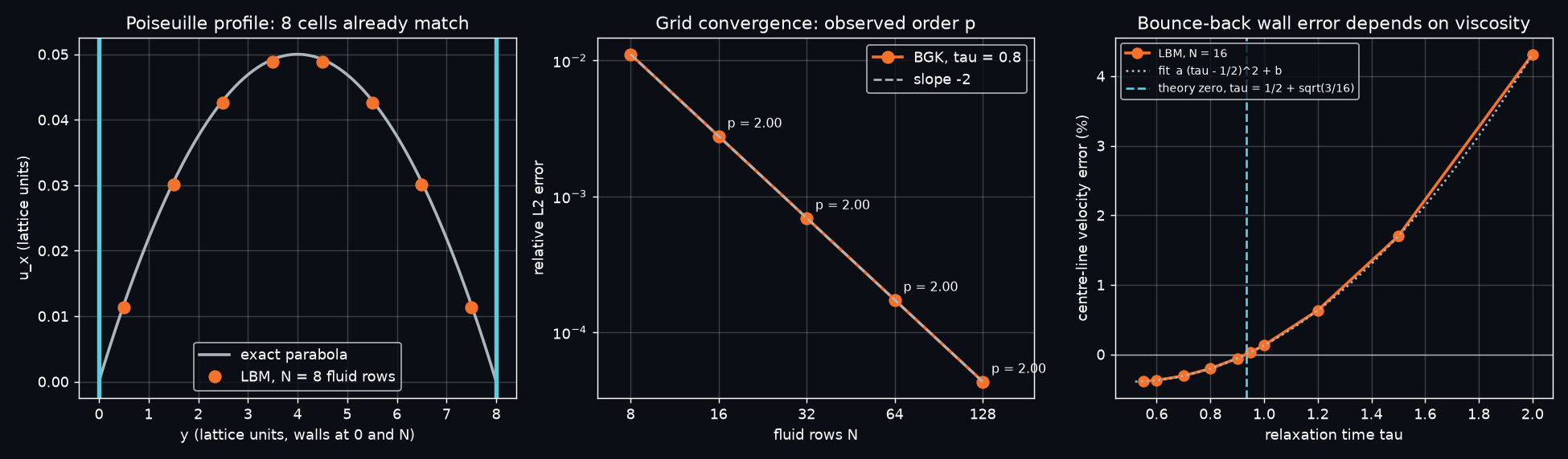
A body-force-driven channel (Guo forcing, BGK, τ = 0.8) between half-way bounce-back walls, run to a steady state (update < 10⁻¹² u_max), compared with the exact parabola $u(y)=4u_{max}\,y(N-y)/N^2$:
| fluid rows N | 8 | 16 | 32 | 64 | 128 |
|---|---|---|---|---|---|
| relative L2 error | 1.112e-2 | 2.781e-3 | 6.954e-4 | 1.738e-4 | 4.346e-5 |
| observed order p | 2.000 | 2.000 | 2.000 | 2.000 |
- Exactly second order, which is what the theory promises for grid-aligned walls. With only 8 cells across the channel the profile is already within 1.1 %.
- Right panel: the error has a known structure. For BGK with half-way bounce-back, the wall sits slightly off the half-way point, by an amount that depends on viscosity (He et al. 1997). The centre-line error runs from about −0.4 % at τ = 0.55 to +4.3 % at τ = 2. A fit linear in (τ − ½)² puts the zero at τ = 0.9330, and theory says ½ + √(3/16) = 0.9330. This is the famous "magic" value; TRT collision (Ginzburg) makes the wall exact for every τ.
- Lesson. A verification test run at τ = 0.933 would pass for the wrong reason. Test more than one parameter value.
6.2 Solution verification + benchmark: Schäfer–Turek 2D-2
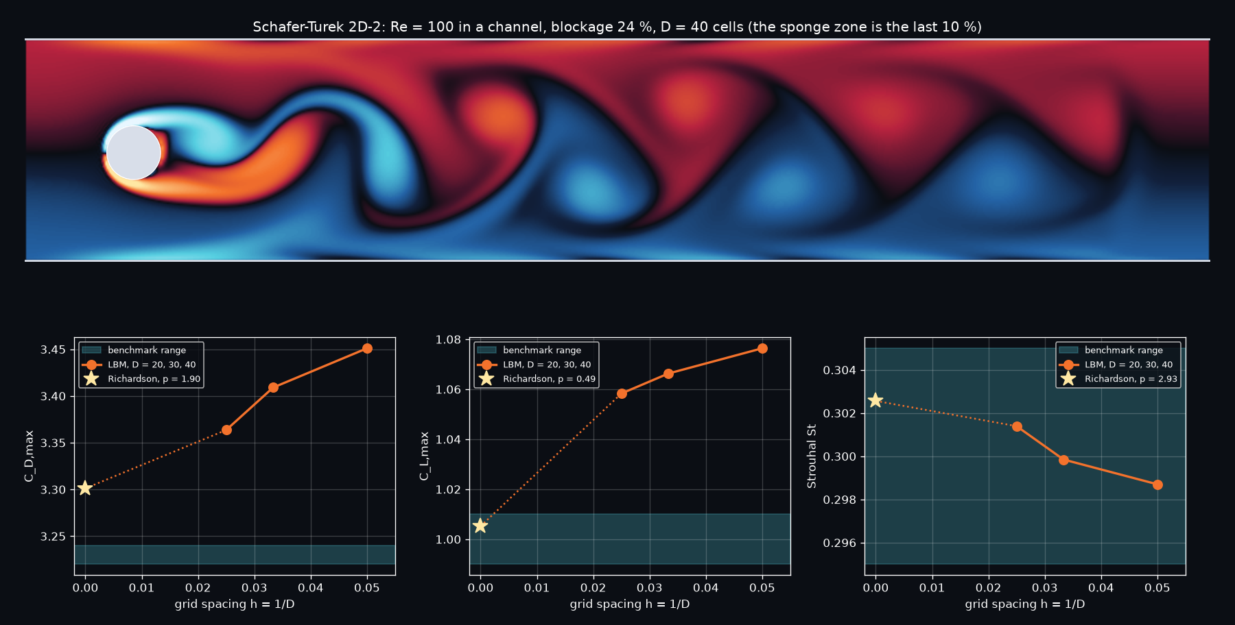
The international laminar benchmark (Schäfer & Turek 1996): cylinder in a channel of height 4.1 D, slightly off-centre, parabolic inflow, Re = 100, 24 % blockage. Three grids, Grid Convergence Index per Celik et al. (2008):
| quantity | D = 20 | D = 30 | D = 40 | observed p | Richardson (h → 0) | GCI_fine | benchmark |
|---|---|---|---|---|---|---|---|
| St | 0.2987 | 0.2998 | 0.3014 | 2.93 | 0.3026 | 0.48 % | 0.295–0.305 ✔ |
| C_L,max | 1.0764 | 1.0663 | 1.0583 | 0.49 | 1.0052 | 6.27 % | 0.99–1.01 ✔ |
| C_D,max | 3.4510 | 3.4091 | 3.3636 | 1.90 | 3.3011 | 2.32 % | 3.22–3.24 ✘ (+2 %) |
| C_D,mean | 3.3867 | 3.3542 | 3.3132 | 2.60 | 3.2764 | 1.39 % | (not tabulated) |
- St is inside the benchmark band on every grid. The zero-crossing estimate agrees with the FFT to 4 digits (0.3014 / 0.3014).
- C_L,max converges into the band (Richardson 1.005). C_D,max does not: it extrapolates to 3.301, 2 % high. The compressibility study (§6.4) finds that Ma = 0.17 inflates C_D by +3.1 %. Divide that out and C_D,max ≈ 3.20, within 0.6 % of the band and inside our own GCI. The Mach correction was measured on C_D,mean and applied to C_D,max, which is an approximation.
- The observed orders (0.5–2.9) are all over the place. That is the signature of a first-order, staircase boundary: the effective cylinder shape changes non-smoothly as D grows, and τ changes too (0.54 → 0.58, because U is fixed). This is exactly why Celik's procedure reports p instead of assuming it.
- The organ-pipe bug. The first version had no sponge. C_D,max came out at 3.65 at D = 20 because ±0.1 of acoustic ringing rode on the ±0.035 physical oscillation: the tunnel's quarter-wave mode, period 4L/c_s ≈ 3050 steps, which was also visible in the spectrum. LBM is weakly compressible, so every closed tunnel is a musical instrument. A 10 % absorbing layer cleaned the signal (the drag trace is now a pure 2f sine), without changing St.
6.3 Validation: a cylinder in free stream vs experiment
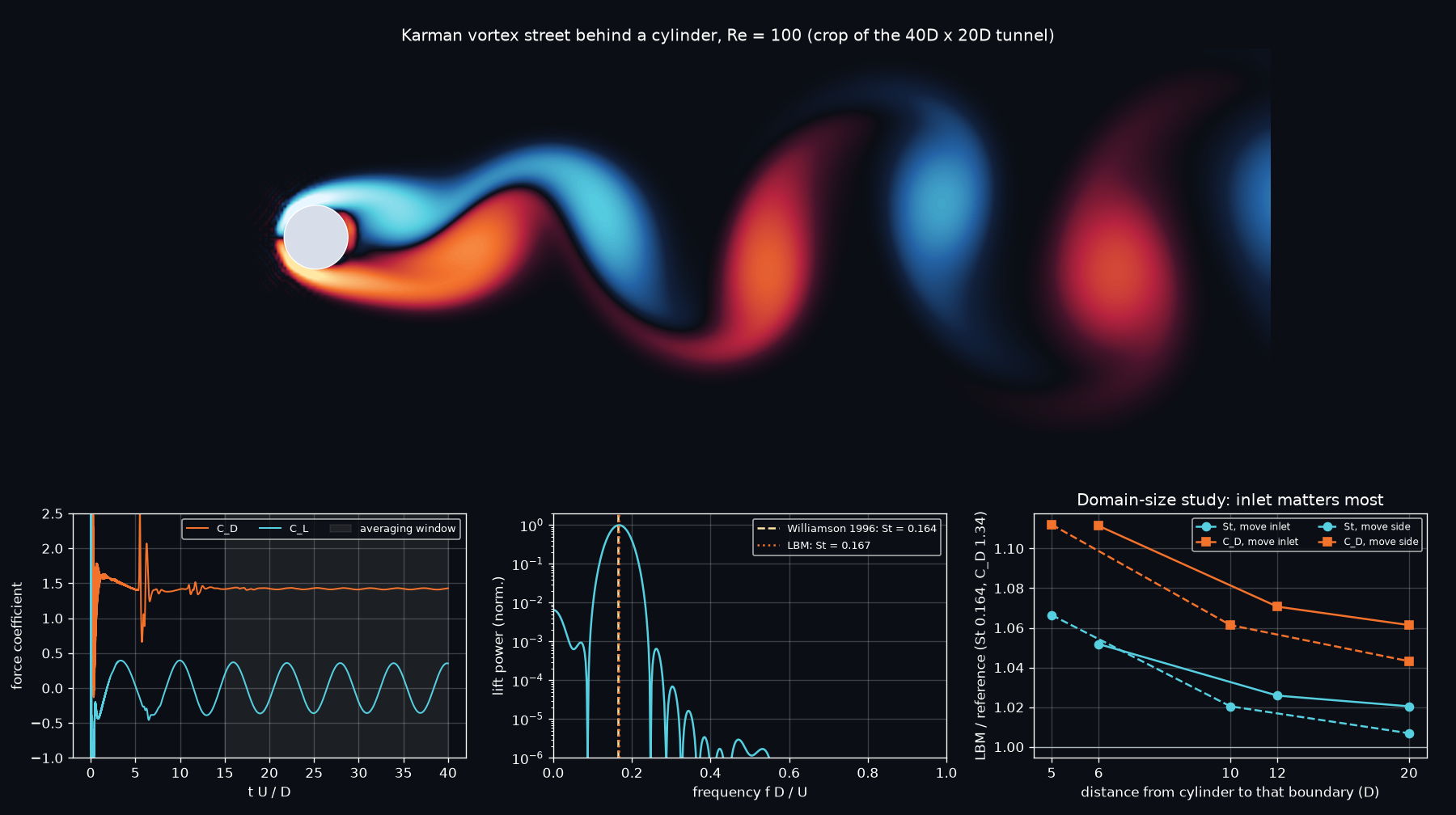
Re = 100, D = 20 cells, uniform inflow, periodic sides with absorbing bands. The reference values are Williamson's (1996) measured Strouhal number, St = 0.164, and well-resolved unconfined simulations for the forces: C_D = 1.33–1.35, lift amplitude 0.33–0.34 (Park et al. 1998; Liu et al. 1998).
Domain-size study (move one boundary at a time):
| inlet upstream | sides apart | St | C_D | C_L amplitude |
|---|---|---|---|---|
| 6 D | 20 D | 0.1725 | 1.4894 | 0.391 |
| 12 D | 20 D | 0.1682 | 1.4347 | 0.371 |
| 20 D | 20 D | 0.1674 | 1.4223 | 0.367 |
| 20 D | 10 D | 0.1749 | 1.4902 | 0.369 |
| 20 D | 40 D | 0.1651 (+0.7 %) | 1.3979 (+4 %) | 0.362 (+7 %) |
Error budget for the largest tunnel, using the other studies in this level:
| C_D | St | |
|---|---|---|
| largest tunnel (D = 20, Ma = 0.139) | 1.3979 | 0.1651 |
| ÷ grid factor (D = 20 vs Richardson, from §6.2, same D and Re) | ÷ 1.0337 | ÷ 0.9872 |
| ÷ compressibility factor (Ma² fit, §6.4) | ÷ 1.0200 | ÷ 1.0036 |
| best estimate | 1.3258 (refs 1.33–1.35) | 0.1667 (Williamson 0.164, +1.6 %) |
Applying the Schäfer–Turek grid factor for C_L,max (1.0764/1.0052 = 1.071) to the lift amplitude gives 0.362/1.071 = 0.338, inside the 0.33–0.34 references. All three quantities close to within ~2 % once each error source has been measured, not guessed.
The honest part of this story. The first validation run (inlet 6 D upstream) gave St +5.2 % and C_D +11 %. We suspected blockage and ran sides 10 D and 20 D apart. A straight-line extrapolation of those two points to zero blockage gave St = 0.1650, +0.6 % from Williamson: the right answer for the wrong reason. A third point (sides 40 D apart) barely moved (0.1718), so the extrapolation was fiction. Moving the inlet was what mattered: a velocity inlet 6 D upstream sits in the cylinder's own displacement field and forces the oncoming flow. Two-point extrapolations cannot detect curvature. Always refine until the answer stops moving.
6.4 Where the method runs out: stability and compressibility
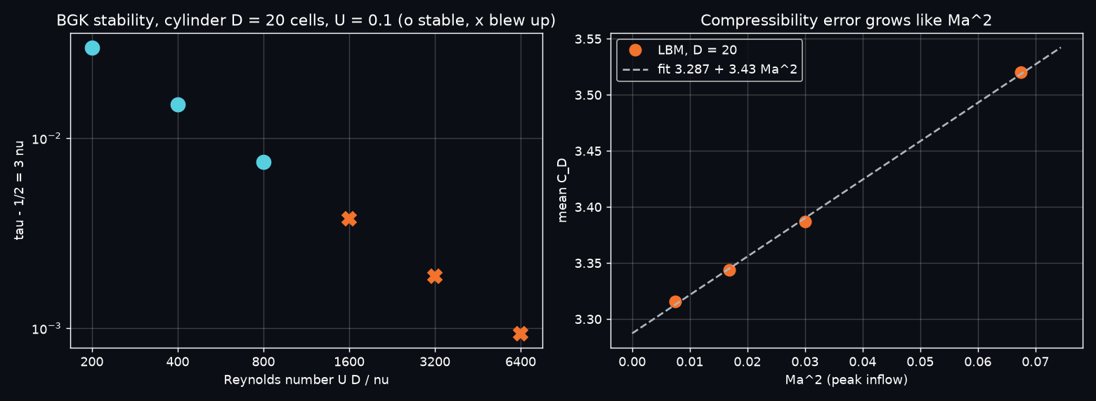
- BGK stability (cylinder D = 20, U = 0.1): stable at Re = 200, 400, 800 (τ − ½ = 0.03, 0.015, 0.0075). Blows up at Re = 1600, 3200, 6400 (τ − ½ ≤ 0.00375). As τ → ½ the viscosity → 0, and BGK's non-hydrodynamic modes stop being damped.
- Compressibility: four Mach numbers on Schäfer–Turek at D = 20. C_D,mean = 3.3158, 3.3442, 3.3867, 3.5200 at peak Ma = 0.087, 0.130, 0.173, 0.260. That is a clean C_D = 3.287 + 3.43 Ma²: +3.1 % at Ma = 0.17, while St moves by only ≈ 0.5 %. Halving U cuts the error 4× but doubles the number of steps.
The Reynolds number a laptop LBM can reach, honestly. With N cells across the body, $\mathrm{Re} = UN/\nu = 3UN/(\tau-\tfrac12)$. Accuracy caps U at ≈ 0.1 (Ma ≈ 0.17, a few % error), and BGK stability caps τ − ½ at ≈ 0.004–0.008 on this kind of geometry. Together that gives Re ≲ 40–80 × N: about 1000 for our 20-cell cylinder, and a few thousand for a 64–128-cell airfoil. Going further costs: at fixed Ma and τ, N ∝ Re and the steps ∝ N/U, so 2D work ∝ Re³ (3D ∝ Re⁴). A Re = 10⁶ airfoil resolving only a laminar boundary layer (δ ≈ 5c/√Re) needs c ≈ 2000 cells, ~2×10⁸ nodes (14 GB) and ~6×10¹³ updates: days on this machine. And real flow at that Re is 3D and turbulent. This is why PowerFLOW uses VLES turbulence modelling, wall functions and octree refinement. The eddy viscosity also raises the effective τ, which keeps BGK-type schemes stable at Re = 10⁷.
6.5 Showcase: NACA 0012 at Re = 1000
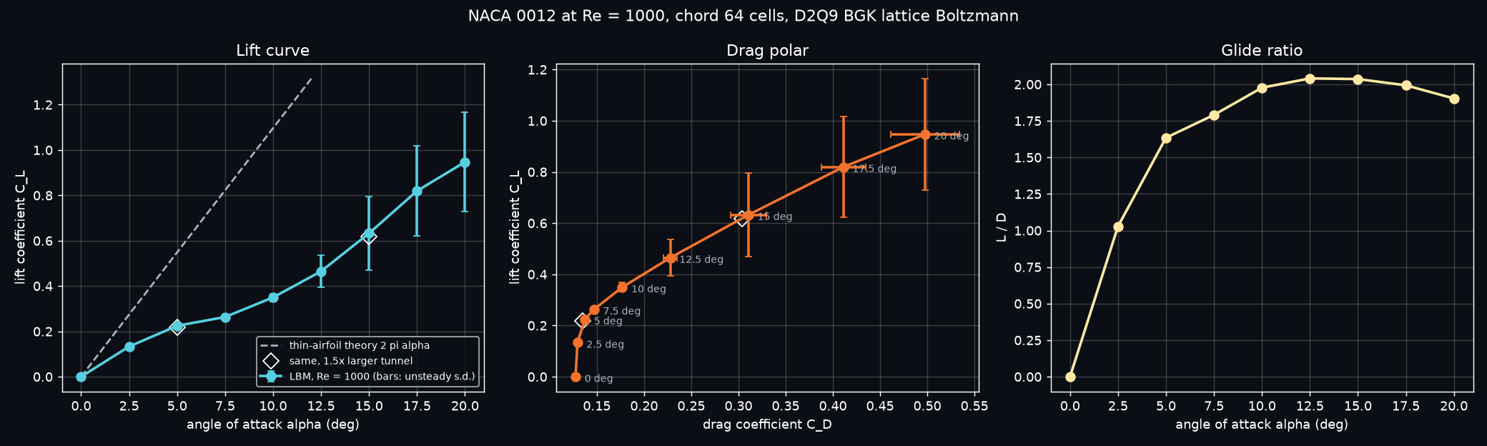
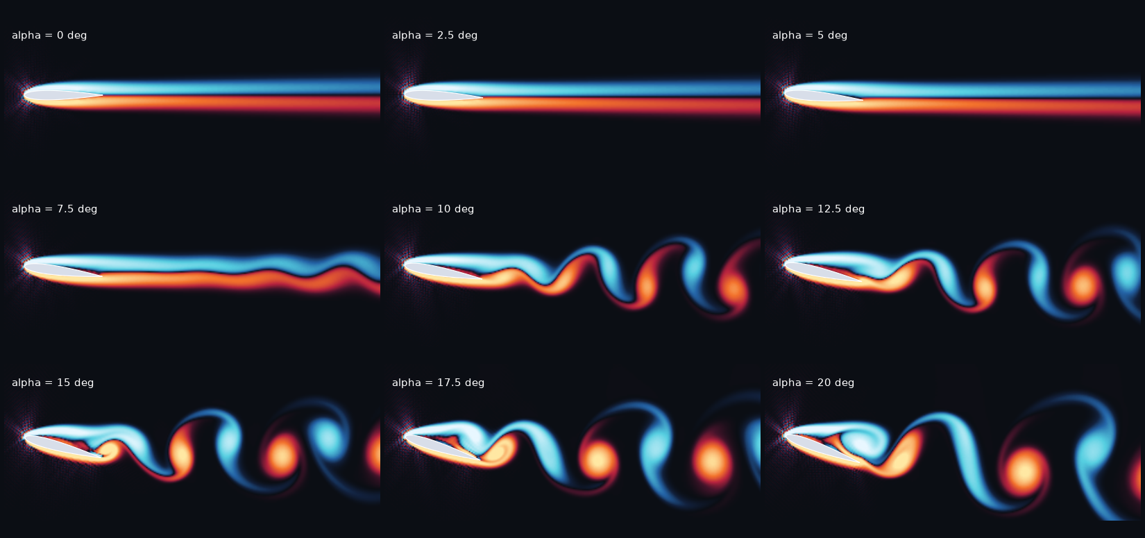
Chord 64 cells, tunnel 10c × 5c, spin-up 10 c/U, then averaging over 6 c/U (bars: s.d. of the unsteady force):
| α (deg) | C_L | ±s.d. | C_D | L/D | St_c = f c/U | St_h = f c sin α / U |
|---|---|---|---|---|---|---|
| 0 | 0.000 | 0 | 0.127 | 0 | steady | |
| 2.5 | 0.133 | 0 | 0.129 | 1.03 | steady | |
| 5 | 0.225 | 0.001 | 0.137 | 1.63 | steady | |
| 7.5 | 0.263 | 0.002 | 0.147 | 1.79 | steady | |
| 10 | 0.350 | 0.018 | 0.177 | 1.98 | weak oscillation | |
| 12.5 | 0.465 | 0.071 | 0.228 | 2.04 | 0.781 | 0.169 |
| 15 | 0.633 | 0.162 | 0.311 | 2.04 | 0.708 | 0.183 |
| 17.5 | 0.820 | 0.198 | 0.411 | 1.99 | 0.635 | 0.191 |
| 20 | 0.947 | 0.218 | 0.498 | 1.90 | 0.562 | 0.192 |
- Viscosity rules at Re = 1000. The small-angle lift slope is 3.05 per radian, 0.49 × the 2π of thin-airfoil theory (the Re → ∞, inviscid limit). Thick laminar boundary layers de-camber the section. C_D at 0° is 0.127. Laminar skin friction alone (Blasius, both sides, 2 × 1.328/√Re) is 0.084, so about ⅔ of the drag is friction and ⅓ is pressure (form) drag. Max L/D ≈ 2, where an airliner wing at Re ~ 10⁷ reaches ≈ 20.
- No classic stall. The lift curve flattens around 7.5° as the trailing-edge separation grows. Shedding starts near 10°, and lift then rises faster again: vortex lift from the separated shear layer, the mechanism insects use. The forces oscillate by up to ±0.22.
- Past 12.5° the wing sheds like a bluff body. Using the projected height c sin α, the Strouhal number collapses to 0.17–0.19. That is the universal bluff-body range; Fage & Johansen (1927) measured ≈ 0.15 for flat plates at high incidence and much higher Re. This is a consistency check, not a validation.
- Domain check (the cylinder's lesson applied). In a 1.5× larger tunnel (15c × 7.5c), α = 5° gives C_L 0.219 (−2.7 %) and C_D 0.135 (−1.8 %). α = 15° gives C_L 0.617 (−2.5 %) and C_D 0.304 (−2.2 %). A first sweep in a 7c × 3.5c tunnel was 6–8 % high, so the tunnel was enlarged and the sweep rerun.
- Grid check (movie tunnel 7.8c × 3.5c, α = 20°): chord 64 gives C_L = 1.009, C_D = 0.530. Chord 128 gives C_L = 1.050 (+4.0 %), C_D = 0.518 (−2.3 %). The movie's forces are higher than the sweep's because its tunnel is the tight one.
- Known artefact. A faint checkerboard speckle upstream of the leading edge (visible in the gallery at τ = 0.515, almost gone in the hero at τ = 0.531) is BGK's odd–even mode, excited by the staircase nose. It is the same stability issue as §6.4, seen before it blows up. MRT/TRT collision or a finer nose would damp it.
6.6 Engineering notes: what made the kernel fast (measured, 3 threads, shared CPU)
| kernel variant | throughput |
|---|---|
| loop over the 9 directions, wall test inside the loop | ~40 MLUPS (float64) |
walls pre-filled by bounce() (branch-free), still a loop over i with a scratch array |
86–131 MLUPS |
| hand-unrolled 9 directions | 217–443 (float64), 459–889 (float32) |
+ an if store: flag to also write ρ, u inside the loop |
687 → 137 (vectorisation lost) |
| + Guo force terms compiled in (even with g = 0) | 687 → 345 → fixed with a closure constant |
| + sponge fused into the collision | 596 → 102 → kept as a separate pass |
| grid 1024 wide vs 1000 wide | 218 vs 406 (4 kB rows: all 27 input streams hit the same cache sets) |
The production loop (bounce + kernel + inlet/outlet + sponge) ran at 200–530 MLUPS depending on machine load (130–140 on the smallest, overhead-bound 36k-node grid). The lesson: LLVM vectorises simple loops. Any branch or extra live value in the hot loop can cost 2–6×.
6.7 V&V summary (actual printed values)
| check | expected | got | |
|---|---|---|---|
| Poiseuille observed order, N = 8 → 128 | 2 | 2.000, 2.000, 2.000, 2.000 | PASS (asserted) |
| Poiseuille error at N = 16 | < 1 % | 0.278 % | PASS (asserted) |
| bounce-back wall error vanishes at | τ = ½ + √(3/16) = 0.9330 | 0.9330 | PASS (asserted) |
| Schäfer–Turek St, D = 40 | 0.295–0.305 | 0.3014 | PASS (asserted) |
| Schäfer–Turek C_L,max, Richardson | 0.99–1.01 | 1.0052 | PASS |
| Schäfer–Turek C_D,max, Richardson | 3.22–3.24 | 3.3011 (3.20 after the Ma correction) | miss +2 %, explained |
| open cylinder St, largest tunnel | Williamson 0.164 ± 3 % | 0.1651 (+0.7 %) | PASS (asserted) |
| open cylinder C_D, largest tunnel | 1.33–1.35 | 1.3979 (1.326 after the grid + Ma budget) | miss +4 % raw, closes after the budget |
| open cylinder lift amplitude | 0.33–0.34 | 0.362 (0.338 after the grid factor) | miss +7 % raw, closes after the budget |
| airfoil domain convergence (1.5× tunnel) | small | −1.8 … −2.7 % | reported |
| airfoil grid convergence (chord 64 → 128, α = 20°) | small | +4.0 % C_L, −2.3 % C_D | reported |
| BGK stability, D = 20, U = 0.1 | – | stable τ − ½ ≥ 0.0075, blows up ≤ 0.00375 | reported |
7. Run it
# from SimulationLab/
uv run python L06_virtual_wind_tunnel/sim.py            # full run
uv run python L06_virtual_wind_tunnel/sim.py --quick    # smoke test: fewer grids, angles and frames
Runtime. The final full run took 5.7 min (341 s) on the 8-core dev machine (3 Numba threads, CPU shared
with other simulations). The main costs are the domain study (~50 s), the airfoil sweep + domain checks (~2 min)
and the movie (~2 min, half of it rendering). --quick takes about 1.3 min. The solver is deterministic (no
random numbers, no parallel reductions), so the numbers reproduce exactly; only MLUPS vary with machine load.
Outputs go to output/: hero.png, wind_tunnel.mp4, verify_poiseuille.png, validate_schafer_turek.png,
validate_cylinder.png, limits.png, airfoil_polar.png, airfoil_gallery.png. The script raises
AssertionError if a verification check fails.
8. Code tour (sim.py)
| Function | What it does |
|---|---|
_make_stream_collide(forced) → stream_collide, stream_collide_forced |
the solver: fused pull-stream + BGK collision, hand-unrolled over the 9 directions, prange over rows. forced is a closure constant, so the Guo body-force terms are compiled out of the wind-tunnel version |
bounce(f, links, body) |
half-way bounce-back written into the solid nodes the pull reads from (so the main loop has no wall branches), plus the momentum-exchange force |
find_links(solid, body) |
every (direction, fluid node, solid node) link, found once with np.roll |
edges, feq |
non-equilibrium-extrapolation velocity inlet and pressure outlet |
sponge, sponge_profile |
absorbing layer at the outlet and open sides |
_curl (@stencil), vorticity |
the vorticity as a numba.stencil relative-index kernel |
simulate(...) |
the time loop: bounce → stream/collide → edges → sponge, with force history and an on_frame callback for the movie |
moments, equilibrium |
populations ↔ (ρ, u) |
spectrum, zero_cross_period |
Hann-windowed zero-padded scipy.fft spectrum; independent period estimate |
disk, naca00xx, polygon_mask, tunnel_start |
geometry (NACA 4-digit formula, rotated about the quarter chord) and the kicked impulsive start |
poiseuille, verify_poiseuille |
code verification: steady channel, observed order, wall error vs τ |
cylinder_run, schafer_turek, open_cylinder |
the cylinder experiments and their force/Strouhal post-processing |
gci |
Celik et al. (2008) three-grid procedure with unequal refinement ratios |
validate_cylinders |
the grid study, benchmark comparison, validation run and their two figures |
limits |
BGK blow-up probe and the Mach-number sensitivity study |
airfoil_tunnel, airfoil_sweep, polar_figures |
the NACA 0012 sweep, polar and gallery |
showcase_movie |
high-resolution stalled-airfoil run rendered frame by frame into the MP4, then hero.png |
verify |
the assertions; main runs everything in order and prints timings |
9. Simplifications & ceilings
- 2D and laminar. A real cylinder wake turns three-dimensional near Re ≈ 190 (Williamson's mode A), so 2D at Re = 100 is physical. A wing at Re = 1000 and 20° would develop spanwise structure in 3D, and 2D over-predicts the force oscillations there. Going to 3D means D3Q19 (19 populations per node) and a third grid dimension, so memory and work grow by the spanwise cell count: ~100× for a modest span.
- BGK collision (
ponytail:instream_collide). One relaxation time for every moment. It is unstable as τ → ½ (§6.4) and leaves the leading-edge checkerboard. Upgrades: TRT (the magic Λ = 3/16 makes bounce-back exact for every τ), MRT, regularised or cumulant collision. - Staircase half-way bounce-back (
ponytail:inbounce). First order on curved walls; the effective body surface is uncertain by a fraction of a cell. This is likely the main source of the D = 20 grid error (C_D +3.4 %). Upgrade: Bouzidi interpolated bounce-back, or immersed boundaries. - Weakly compressible. Ma = 0.14–0.17 in every tunnel run gives +2–3 % on drag (measured). The fix is smaller U at proportionally more time steps.
- Uniform grid (
ponytail:insimulate). The cells far from the body are as fine as the cells in the boundary layer, so most of the work is spent where nothing happens. Upgrade: octree refinement with rescaled τ per level, PowerFLOW's "VR regions". - Simple sponge + extrapolation boundaries (
ponytail:insponge_profile). They still reflect a little; the startup pressure pulse is visible bouncing off the inlet in the cylinder's force trace at t ≈ 5 D/U. Upgrade: characteristic (non-reflecting) boundary conditions, and a smooth start. - Periodic sides. The "free stream" is really an infinite column of bodies, one every H. Damped by the absorbing bands and quantified by the domain studies, but not zero: the sides still moved St by 1.4 % from 20 D to 40 D apart.
- The error budget transfers a grid factor from the confined Schäfer–Turek cylinder to the open one (same D, same Re, same staircase). That is plausible, but it is an estimate; a direct D = 30/40 open-cylinder study would replace it (Go further 1).
- Short averaging windows (15–25 D/U for the cylinders, 6 c/U for the airfoil) keep the run under 6 minutes. That is enough for periodic shedding. It is marginal for the irregular high-α airfoil, where the s.d. bars show the spread.
10. Go further
- Rebuild it in OpenFOAM. Mesh the Schäfer–Turek channel with
blockMesh(an O-grid around the cylinder), runpimpleFoamat Re = 100 with theforceCoeffsfunction object, and put your C_D,max, C_L,max and St in the same GCI table. Then compare wall-clock time and engineer time (meshing!) with this LBM. - Interpolated bounce-back (Bouzidi et al. 2001). Use the exact wall distance q along each link instead of assuming ½. This should turn the first-order cylinder convergence of section 6 into second order and pull C_D onto the benchmark at D = 20. It also removes most of the leading-edge checkerboard.
- TRT or MRT collision. Two-relaxation-time with the magic parameter Λ = 3/16 makes the Poiseuille wall error vanish for every τ (not just τ = 0.933), and MRT/regularised/cumulant operators push the stability floor well below our BGK limit (τ − ½ ≈ 0.004–0.008, §6.4). How high can you take the airfoil's Re before it blows up?
- Compare with XFOIL. Run
xfoilon NACA 0012 at Re = 10⁴, 10⁵, 10⁶ and plot its polars on top of ours at Re = 1000. Watch the lift slope climb towards 2π and the drag fall by an order of magnitude. Then push the LBM to the highest Re it survives and see where the two start to meet. - Go 3D on a GPU. Port
stream_collideto D3Q19 with CuPy or Numba-CUDA (the same stencil, one thread per node) and simulate a sphere at Re = 300 (where its wake becomes unsteady), or a 3D wing tip vortex. That is the first step towards what PowerFLOW does on 10⁹ voxels.
11. References
- T. Krüger, H. Kusumaatmaja, A. Kuzmin, O. Shardt, G. Silva, E. M. Viggen, The Lattice Boltzmann Method: Principles and Practice (Springer, 2017). The textbook; chapters 5 (boundaries), 6 (forces) and 11 (MRT/TRT) back most of this code.
- S. Succi, The Lattice Boltzmann Equation: For Complex States of Flowing Matter (Oxford, 2018).
- Y. H. Qian, D. d'Humières, P. Lallemand, "Lattice BGK models for Navier–Stokes equation," Europhys. Lett. 17, 479 (1992).
- S. Chen, G. D. Doolen, "Lattice Boltzmann method for fluid flows," Annu. Rev. Fluid Mech. 30, 329 (1998).
- A. J. C. Ladd, "Numerical simulations of particulate suspensions via a discretized Boltzmann equation. Part 1," J. Fluid Mech. 271, 285 (1994). Bounce-back and momentum exchange.
- X. He, Q. Zou, L.-S. Luo, M. Dembo, "Analytic solutions of simple flows and analysis of nonslip boundary conditions for the lattice Boltzmann BGK model," J. Stat. Phys. 87, 115 (1997). The τ-dependent bounce-back wall error.
- I. Ginzburg, D. d'Humières, "Multireflection boundary conditions for lattice Boltzmann models," Phys. Rev. E 68, 066614 (2003).
- Z. Guo, C. Zheng, B. Shi, "Discrete lattice effects on the forcing term in the lattice Boltzmann method," Phys. Rev. E 65, 046308 (2002); and "Non-equilibrium extrapolation method for velocity and pressure boundary conditions in the lattice Boltzmann method," Chinese Physics 11, 366 (2002).
- M. Bouzidi, M. Firdaouss, P. Lallemand, "Momentum transfer of a Boltzmann-lattice fluid with boundaries," Phys. Fluids 13, 3452 (2001).
- P. Lallemand, L.-S. Luo, "Theory of the lattice Boltzmann method: dispersion, dissipation, isotropy, Galilean invariance, and stability," Phys. Rev. E 61, 6546 (2000).
- M. Schäfer, S. Turek, "Benchmark computations of laminar flow around a cylinder," in Flow Simulation with High-Performance Computers II, Notes on Numerical Fluid Mechanics 52, 547 (Vieweg, 1996).
- C. H. K. Williamson, "Vortex dynamics in the cylinder wake," Annu. Rev. Fluid Mech. 28, 477 (1996).
- J. Park, K. Kwon, H. Choi, "Numerical solutions of flow past a circular cylinder at Reynolds numbers up to 160," KSME Int. J. 12, 1200 (1998).
- C. Liu, X. Zheng, C. H. Sung, "Preconditioned multigrid methods for unsteady incompressible flows," J. Comput. Phys. 139, 35 (1998).
- A. Fage, F. C. Johansen, "On the flow of air behind an inclined flat plate of infinite span," Proc. R. Soc. A 116, 170 (1927).
- P. J. Roache, Verification and Validation in Computational Science and Engineering (Hermosa, 1998).
- I. B. Celik et al., "Procedure for estimation and reporting of uncertainty due to discretization in CFD applications," J. Fluids Eng. 130, 078001 (2008).
- W. L. Oberkampf, C. J. Roy, Verification and Validation in Scientific Computing (Cambridge, 2010); ASME V&V 20-2009.
- T. Colonius, "Modeling artificial boundary conditions for compressible flow," Annu. Rev. Fluid Mech. 36, 315 (2004). Sponge layers and why tunnels ring.
- H. Chen, S. Kandasamy, S. Orszag, R. Shock, S. Succi, V. Yakhot, "Extended Boltzmann kinetic equation for turbulent flows," Science 301, 633 (2003). The physics behind PowerFLOW's VLES.
- M. Drela, "XFOIL: An analysis and design system for low Reynolds number airfoils," in Low Reynolds Number Aerodynamics, Lecture Notes in Engineering 54, 1 (Springer, 1989).