Level 7 of 10 · Climate science

VERIFIEDTransient climate response 1.60 [1.42, 1.80] K, inside the IPCC AR6 range. Recovers 10/10 synthetic truths; 93% of observations fall in the 90% band.

L07: Earth's Thermostat

Real data meets the model. We take a two-box climate model, fit it to 146 years of NASA temperature records with Markov chain Monte Carlo, and ask how much the past really tells us about the future. The model is small enough to run a million times. The past record, it turns out, pins down one number well (the transient response) and leaves the one people care about most (equilibrium sensitivity) mostly to the priors.

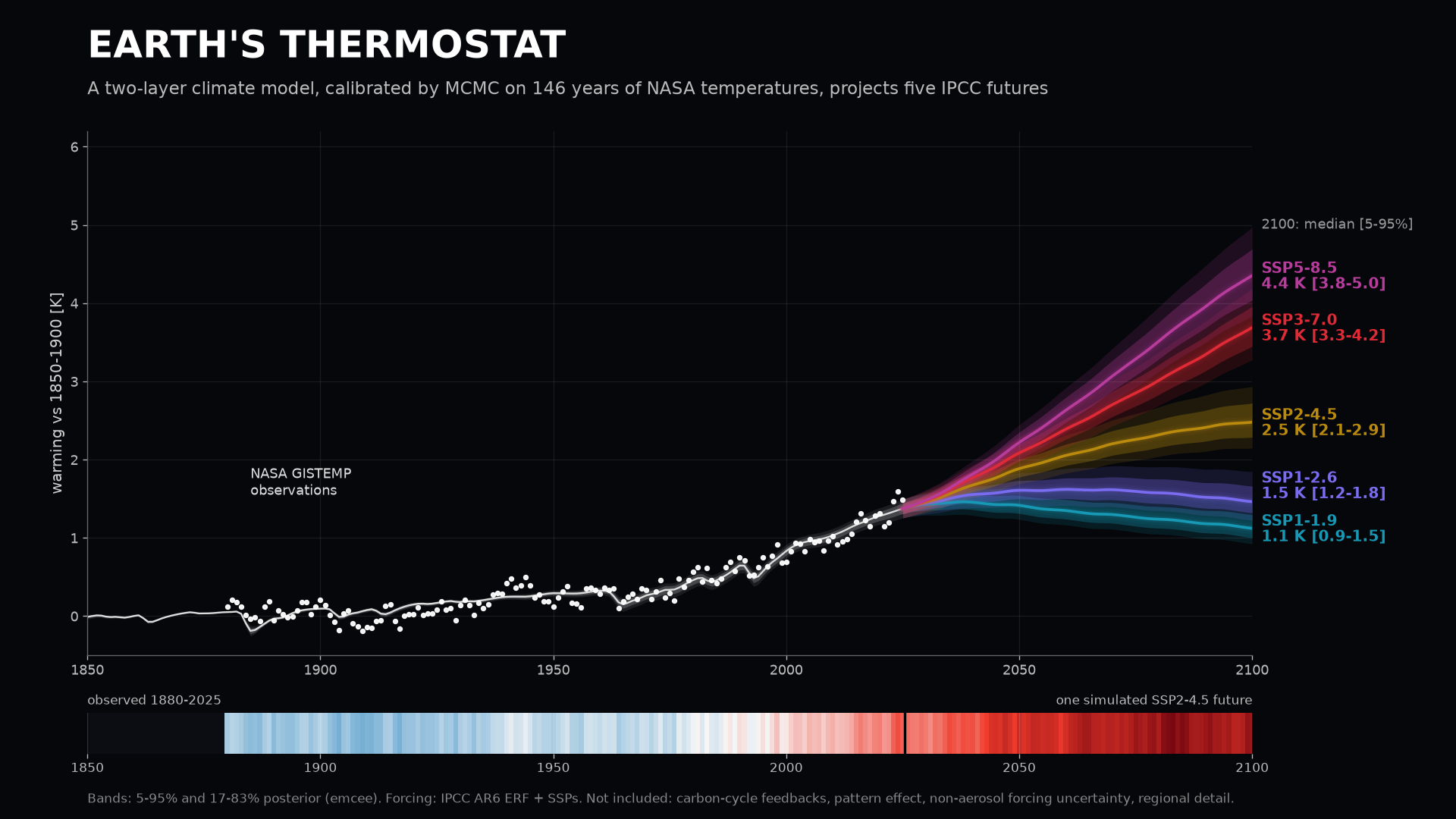
hero

Movie: output/mcmc_walkers.mp4 (1280×600, 8 s, H.264). 64 emcee walkers start from random prior draws and climb onto the posterior. Left: each walker's (ECS, aerosol scale), with the final posterior as white contours. Right: each walker's simulated climate against NASA GISTEMP.

1. The question

Doubling CO₂ adds about 3.9 W m⁻² of energy to the climate system. How much warmer does the planet get? Two numbers summarise the answer:

ECS (equilibrium climate sensitivity): the warming once the deep ocean has caught up, centuries later.
TCR (transient climate response): the warming at the moment of doubling when CO₂ rises 1 %/yr. It is roughly what we live through this century.

IPCC AR6 (2021) assessed ECS at 3 K (likely 2.5 to 4 K) and TCR at 1.8 K (likely 1.4 to 2.2 K), combining process understanding, paleoclimate, the historical record and models. This level uses only the historical record plus physically motivated priors, and turns the question into a calibration problem:

Which parameter values of a simple energy-balance model are consistent with observed warming, given realistic, autocorrelated year-to-year noise?
How do we know the sampler and the likelihood are working? (diagnostics, posterior predictive checks, synthetic-truth recovery, coverage)
Which parameters actually drive the uncertainty, in the past and in 2100? (Sobol vs one-at-a-time)
What does the calibrated model project for the five IPCC SSP scenarios, and what can such a model not say?

2. The model

Two-layer energy balance (Held et al. 2010; Geoffroy et al. 2013a). A mixed layer (atmosphere, land and upper ocean) with temperature $T$ sits on a deep ocean with temperature $T_d$:

$$C\,\frac{dT}{dt} = F(t) - \lambda T - \gamma\,(T - T_d), \qquad C_d\,\frac{dT_d}{dt} = \gamma\,(T - T_d)$$

$$F(t) = F_{\text{non-aer}}(t) + \alpha_{aer}\,F_{aer}(t)$$

Symbol	Meaning	Units
$\lambda$	climate feedback parameter (how fast extra heat radiates away)	W m⁻² K⁻¹
$\gamma$	heat exchange between the layers	W m⁻² K⁻¹
$C,\ C_d$	heat capacities of the mixed layer and deep ocean	W yr m⁻² K⁻¹ (1 unit ≈ 7.7 m of seawater over the whole globe)
$\alpha_{aer}$	scale factor on the IPCC aerosol forcing (the most uncertain forcing)	1

Derived quantities: $\text{ECS} = F_{2\times}/\lambda$ with $F_{2\times}=3.93$ W m⁻² (AR6). TCR is the mean warming over years 61 to 80 of a 1 %/yr CO₂ ramp. The Earth's energy imbalance is $N = F - \lambda T$. The system has two e-folding modes: a fast one (years, the mixed layer) and a slow one (centuries, the deep ocean).

Exact integration. The model is linear, $\dot{\mathbf x} = A\mathbf x + B F$. With annual forcing held constant over each year, the one-year map $\mathbf x_{n+1} = e^{A}\mathbf x_n + A^{-1}(e^{A}-I)B\,F_n$ is exact. $e^A$ comes from Sylvester's formula for a 2×2 matrix with real eigenvalues, written out in closed form inside a Numba kernel. There is no time-step error, and one run of 1750 to 2100 costs a few microseconds per parameter set.

Statistical model. Observed anomaly = model + baseline offset + AR(1) noise:

$$y_t = T_t(\theta) + T_0 + r_t, \qquad r_t = \rho\, r_{t-1} + e_t,\quad e_t\sim\mathcal N(0,\sigma^2)$$

The exact AR(1) likelihood draws $r_1$ from the stationary law $\mathcal N(0,\sigma^2/(1-\rho^2))$ and whitens the rest: $e_t = r_t - \rho r_{t-1}$. AR(1) "red noise" is Hasselmann's (1976) picture of weather forcing a slow ocean. It lumps internal variability (ENSO and the rest), measurement error and model error into one process.

Priors (8 parameters):

Parameter	Prior	Why
$\lambda$	Uniform(0.2, 4)	broad; implies an ECS prior of 1 to 20 K, heavy toward low ECS (∝ 1/ECS²)
$\gamma,\ C,\ C_d$	lognormal centred on 35 CMIP6 two-layer fits (AR6 Ch. 7 data), log-spread ×2	medians 0.60, 8.1, 99; physics from climate models, widened because an ensemble shares biases
$\alpha_{aer}$	Normal(1, 0.35), truncated to [0, 3]	AR6 aerosol ERF 1750-2019 is −1.1 [−1.7, −0.4] W m⁻²
$T_0$	Uniform(−1, 1) K	baseline offset between GISTEMP (1951-1980) and the model's 1750 zero
$\sigma$	Uniform(0.01, 0.3) K	innovation noise
$\rho$	Uniform(0, 0.95)	lag-1 autocorrelation

Data (downloaded with requests, cached in data/, parsed with pandas):

Source	What	Used for
NASA GISTEMP v4 `GLB.Ts+dSST.csv`	global land+ocean annual anomaly, 1880-2025	the likelihood
IPCC AR6 WG1 Ch. 7 `AR6_ERF_1750-2019.csv`	assessed effective radiative forcing by agent	model input 1750-2019
NOAA Mauna Loa `co2_annmean_mlo.csv`	annual CO₂, 1959-2025	checking AR6 CO₂ forcing against measurements, and extending it to 2020-2025
IPCC Ch. 7 `SSPs/ERF_ssp*_1750-2500.csv`	forcing for SSP1-1.9, 1-2.6, 2-4.5, 3-7.0, 5-8.5	non-CO₂ forcing 2020-2025 (SSP2-4.5), and projections
IPCC Ch. 7 `cmip6_twolayer_tuning_params.csv`	two-layer fits to 35 CMIP6 models	priors on $\gamma, C, C_d$, and the CMIP6 ECS spread

Assumptions. Global means only. Constant feedback $\lambda$ (no pattern effect, no deep-ocean efficacy). Forcing is prescribed (no carbon cycle). Forcing uncertainty enters only through $\alpha_{aer}$. The model starts in equilibrium in 1750.

3. M&S concepts you'll learn here

Calibration as inference. Parameters are not "fitted". They get a posterior distribution $p(\theta\mid y)\propto p(y\mid\theta)\,p(\theta)$, and every downstream number carries that uncertainty.
The likelihood is a noise model. Annual temperature residuals are strongly autocorrelated (ρ ≈ 0.56). Assuming independent residuals shrinks the TCR interval by ~40%, which is overconfidence you can measure.
Ensemble MCMC (emcee). Affine-invariant ensembles need no hand-tuned proposal. Differential-evolution moves beat the default stretch move here.
MCMC diagnostics. Look at trace plots, compute the integrated autocorrelation time τ (and require N > 50τ), check acceptance, and hunt for walkers parked in side modes. Burn-in is a diagnosis, not a constant.
Posterior predictive checks. Replicate the data from the fitted model and ask whether the real record looks like a typical draw: band coverage, test statistics with Bayesian p-values, whitened-residual autocorrelation.
Out-of-sample validation. Earth's energy imbalance is never used in the fit, but the model predicts it. That tests the physics, not just the curve fit.
Synthetic-truth recovery and coverage. Generate fake Earths with known parameters and check that 90% intervals contain the truth about 90% of the time (simulation-based calibration, lite).
Identifiability. A parameter can be "recovered" only because the posterior equals the prior. The ratio sd(post)/sd(prior) shows what the data actually learned.
Degeneracy. Strong aerosol cooling plus high sensitivity fits the same past as weak aerosols plus low sensitivity, but gives different futures.
Global sensitivity analysis. Sobol indices decompose output variance over the whole input space (S₁ = main effect, S_T = with interactions). One-at-a-time answers depend on where you stand.
Projections vs predictions. Scenario projections are conditional on a forcing pathway and a model structure. The fan chart is honest only about the uncertainty that was modelled.

4. Tech stack

Tool	Role here
Python 3.12, NumPy	everything numeric; vectorised likelihood across walkers
Matplotlib (+ ffmpeg via `imageio-ffmpeg`)	all figures (handmade corner plot, trace plots, fan charts) and the MP4
SciPy	`linalg.expm` as the independent check of the integrator; `ndimage.gaussian_filter` to smooth corner-plot contours
Numba	the model kernel: `@njit(parallel=True)`, one `prange` lane per parameter set, 3 threads
★ pandas	parsing four CSV formats (GISTEMP's `***` gaps, NOAA's `#` comments, IPCC's per-agent tables), splicing forcing series by year index, the posterior summary CSV
★ requests	live downloads from NASA, NOAA and GitHub with timeouts and `raise_for_status`, cached to `data/` so reruns work offline
★ emcee	affine-invariant ensemble MCMC with `vectorize=True` (one Numba call per half-ensemble) and `DEMove` + `DESnookerMove`; `get_autocorr_time`, `emcee.autocorr.integrated_time`
★ SALib	Saltelli/Sobol sampling (`SALib.sample.sobol`) and variance-based indices with bootstrap CIs (`SALib.analyze.sobol`); the bundled Ishigami function for verification

SimPy, Mesa and NetworkX from earlier levels are still in the environment but are not needed here. pandas and requests turn "a model" into "a model that eats live data". emcee and SALib turn "a run" into "a distribution of runs you can reason about".

5. Industry & scientific tools

Tool	What it is	Who uses it	How this project maps to it
FaIR (Finite-amplitude Impulse Response)	open-source Python emulator: emissions → concentrations → forcing → a 3-layer EBM	IPCC AR6 WG1 and WG3 (scenario warming classification), many research groups	our `ebm` is FaIR's temperature module with 2 boxes instead of 3. FaIR v2 adds the carbon cycle and calibrates with a constrained ensemble, which is the same Bayesian idea
MAGICC	reduced-complexity climate model, probabilistic set-up	IPCC WG3, IAM teams (IIASA, PIK), NGFS finance scenarios	same role: emulate ESMs cheaply and propagate parameter uncertainty to SSP projections
CMIP6 ESMs (CESM2, E3SM, UKESM, …)	3-D coupled Earth system models on supercomputers	national labs, the CMIP6 archive behind every IPCC figure	our priors come from two-layer fits to these models; the white ticks in the ECS figure are 35 of them
PyMC / Stan	probabilistic programming with gradient-based HMC/NUTS	statistics, epidemiology, pharma, finance	the same posterior written as a model block; NUTS needs gradients (JAX/Stan autodiff through the time loop) but mixes far better in high dimensions
ArviZ	diagnostics and plots for Bayesian inference	PyMC/Stan/emcee users	R-hat, ESS, trace, pair and PPC plots; we hand-roll the emcee-native equivalents (τ, N/50τ, corner, PPC)
Dakota (Sandia)	optimisation, UQ and sensitivity toolkit that wraps any simulation code	DOE labs, aerospace, nuclear	`sampling`, `sobol` and Bayesian calibration (QUESO/DREAM) methods do what our SALib + emcee pipeline does, for expensive black-box models
UQLab (ETH Zürich)	MATLAB UQ framework: surrogates, Sobol, Bayesian inversion	engineering UQ	Sobol via polynomial chaos surrogates: the move when each model run costs hours, not microseconds
OpenTURNS	open-source C++/Python UQ library (EDF, Airbus, Phimeca)	energy and aerospace industry	probabilistic input models, Sobol/Shapley indices, calibration; supports dependent inputs, which our Sobol box ignores

6. Results

All numbers below are printed by sim.py (seed 2021, deterministic).

The data, and a real-data sanity check on the forcing

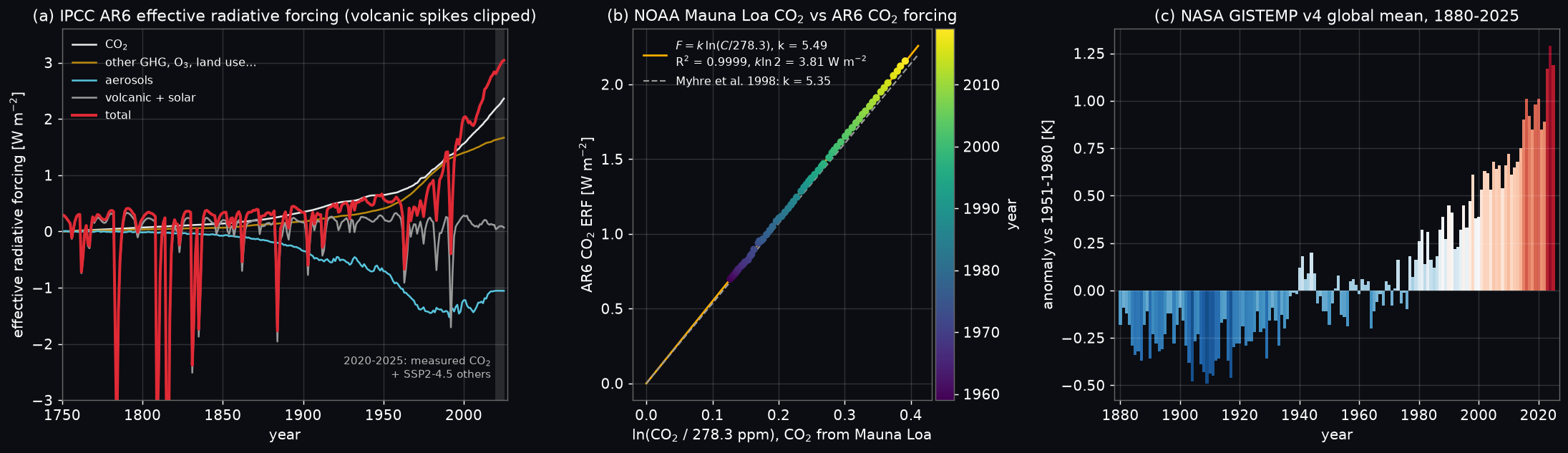
data

(a) Total forcing reached ~2.8 W m⁻² in 2019. Aerosols (blue, −1.06 W m⁻²) mask more than a quarter of the ~3.8 W m⁻² greenhouse-gas and ozone forcing, and that mask is the biggest source of uncertainty in the whole problem. Volcanic eruptions (grey spikes, clipped) are brief but large.
(b) NOAA's measured CO₂ against IPCC's CO₂ forcing. A log law $F = k\ln(C/278.3)$ fitted through the origin gives k = 5.493 W m⁻², R² = 0.99985. That is close to the classic Myhre et al. (1998) 5.35; AR6's value is higher because it includes tropospheric adjustments. The implied $F_{2\times} = k\ln 2 = $ 3.81 W m⁻², inside AR6's 3.93 [3.46, 4.40]. It sits slightly low because the AR6 formula is not purely logarithmic.
The same fit extends CO₂ forcing to 2020-2025 from measurements. That comes out 0.03 to 0.06 W m⁻² below what the SSP2-4.5 scenario assumed. Other agents for 2020-2025 come from SSP2-4.5, which is a scenario, not an observation (see Simplifications).
(c) GISTEMP v4, 1880-2025 (complete calendar years only).

MCMC: 64 walkers × 30 000 steps in 23 s

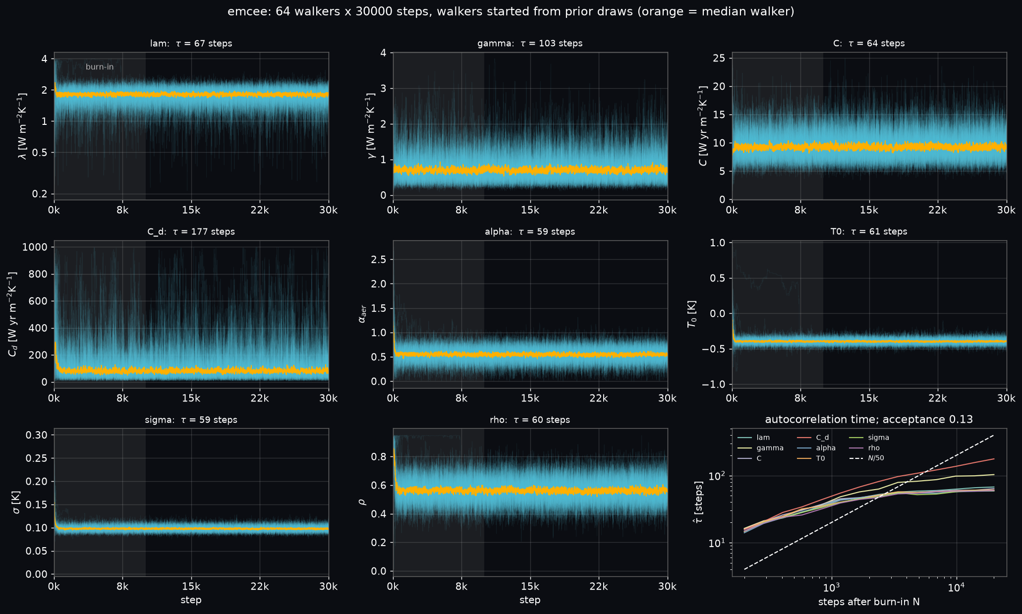
mcmc

Acceptance 0.131 (every walker 0.11 to 0.14). The textbook 0.2 to 0.5 target is for the stretch move. Here we use differential-evolution moves (DEMove 80%, DESnookerMove 20%). In a development test (12 000 steps, earlier and wider prior) they had lower acceptance (0.14 vs 0.40) but shorter autocorrelation times (τ_max 112 vs 169 steps). The quantity that matters is effective samples per second, not acceptance.
Autocorrelation times τ (steps): λ 67, γ 103, C 64, C_d 177, α 59, T0 61, σ 59, ρ 60. The post-burn-in chain is 113 τ_max long (the rule of thumb is > 50), and the τ-vs-N panel shows the estimates flattening once N > 50τ. We keep every 88th step: 14 528 samples.
A walker in a side mode. Walkers start from prior draws on purpose. One of them (walker 33) sat until step 7 364 in a spurious mode with ρ ≈ 0.94, T0 ≈ +0.5 K and λ ≈ 3.9: red noise with near-unit memory "explains" the warming, so the physics does not have to. Its log-probability was far below the ensemble's. With the first burn-in of 4 000 steps it leaked into the posterior as a small bump at ECS ≈ 1 K. The burn-in is now 10 000, and a check asserts that every walker's post-burn-in median log-probability is within 5 units of the ensemble (worst: 0.43).

Posterior (median [5 %, 95 %]; the full table is in output/posterior_summary.csv):

λ [W m⁻²K⁻¹]	γ	C [W yr m⁻²K⁻¹]	C_d	α_aer	T0 [K]	σ [K]	ρ
1.81 [1.29, 2.22]	0.70 [0.33, 1.48]	9.3 [6.4, 13.5]	82 [21, 338]	0.54 [0.31, 0.77]	−0.40 [−0.46, −0.33]	0.098 [0.089, 0.109]	0.56 [0.44, 0.69]

Derived: ECS 2.17 [1.77, 3.04] K, TCR 1.60 [1.42, 1.80] K. The fast mode is 3.6 [2.2, 5.7] yr and the slow mode 169 [38, 822] yr (Geoffroy et al. 2013a found ~4 and ~200+ yr across CMIP5). The implied aerosol forcing in 2019 is −0.58 [−0.82, −0.33] W m⁻², about half of AR6's central −1.1 W m⁻² and in the weak end of its [−1.7, −0.4] range. Simple models fitted to global temperature alone often prefer weak aerosols. With an aerosol-forcing prior this uninformative, the record would rather have a modestly sensitive climate with little masking.

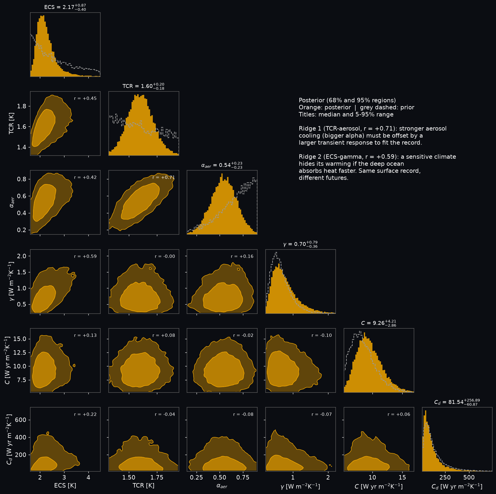
corner

The corner plot (hand-made in matplotlib: 2-D histograms, Gaussian smoothing, 68/95% highest-density contours) shows the two ridges that make climate calibration hard:

TCR vs aerosols (r = +0.64). More aerosol cooling in the past needs a more responsive climate to produce the same warming.
ECS vs γ (r = +0.58). A high-sensitivity climate can hide its warming if the deep ocean takes up heat faster. The surface record cannot tell these apart, but 2100 can.

$C_d$ is essentially its prior (compare the dashed line). 146 years of surface temperature say almost nothing about the deep ocean.

Does the noise model matter? AR(1) vs white noise

The same MCMC with ρ fixed at 0 (independent residuals):

Quantity	AR(1) likelihood	White-noise likelihood	90% width, white / AR(1)
TCR [K]	1.60 [1.42, 1.80]	1.58 [1.47, 1.69]	0.58
α_aer	0.54 [0.31, 0.77]	0.50 [0.36, 0.66]	0.65
T0 [K]	−0.40 [−0.46, −0.33]	−0.41 [−0.44, −0.37]	0.58
ECS [K]	2.17 [1.77, 3.04]	2.21 [1.86, 3.23]	1.08
C	9.3 [6.4, 13.5]	11.3 [7.9, 16.0]	1.13

With autocorrelated residuals, 146 years hold only about 146·(1−ρ)/(1+ρ) ≈ 41 independent pieces of information. The white-noise fit believes it has 146, so the quantities the data really constrain (TCR, aerosol scale, baseline) come out 35 to 42% too narrow. Quantities whose uncertainty comes from the prior and the degeneracies (ECS, C) do not shrink; they shift. Overconfidence hits exactly the numbers you would be tempted to quote.

Posterior predictive checks and an out-of-sample test

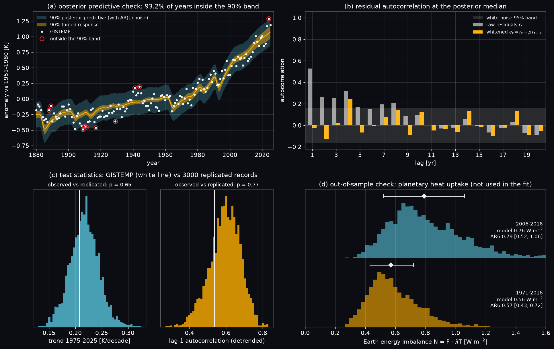
ppc

(a) Coverage. 3 000 replicated records (posterior draw + AR(1) noise). 93.2% of observed years fall inside the 90% predictive band (target 90%). The 10 misses cluster in the 1880s, the unusually cold 1909-1917, the warm early 1940s (a known WWII-era sea-surface-temperature measurement bias plus a strong El Niño) and 2024, the record El Niño year. That year sits above the band because the model's 2020-2025 forcing is a scenario and misses the recent extra warming factors (Simplifications).
(b) Residual autocorrelation. Raw residuals have lag-1 ACF +0.53. Whitening with the posterior ρ brings it to −0.03. Honest miss: lag 4 keeps +0.25, above the white-noise band (±0.16). That is the ENSO quasi-periodicity (3 to 7 yr) that an AR(1) process cannot represent. An ARMA(2,1) or an explicit ENSO index would fix it.
(c) Test statistics. The observed 1975-2025 trend (0.207 K/decade) and the detrended lag-1 autocorrelation (0.54) are typical of replicated records: Bayesian p = 0.65 and 0.77 (bad would be < 0.05 or > 0.95).
(d) Earth's energy imbalance, never used in the fit:

Period	Posterior $N=F-\lambda T$ [W m⁻²]	AR6 assessed (Table 7.1)
1971-2018	0.56 [0.36, 0.90]	0.57 [0.43, 0.72]
2006-2018	0.76 [0.47, 1.28]	0.79 [0.52, 1.06]

The medians agree to within 0.03 W m⁻², which is independent evidence that the calibrated heat uptake is physical. The posterior is wider than AR6's observational range, so adding ocean heat content to the likelihood would sharpen $\gamma$ and $C_d$ (Go further #2).

Warming 2011-2020 vs 1850-1900: forced response 1.17 [1.07, 1.26] K. GISTEMP on the model's baseline gives 1.14 K, against AR6's observed 1.09 [0.95, 1.20] K. In 2025, GISTEMP is at 1.49 K and the forced response at 1.37 K.

Synthetic truth: can the pipeline recover a known Earth?

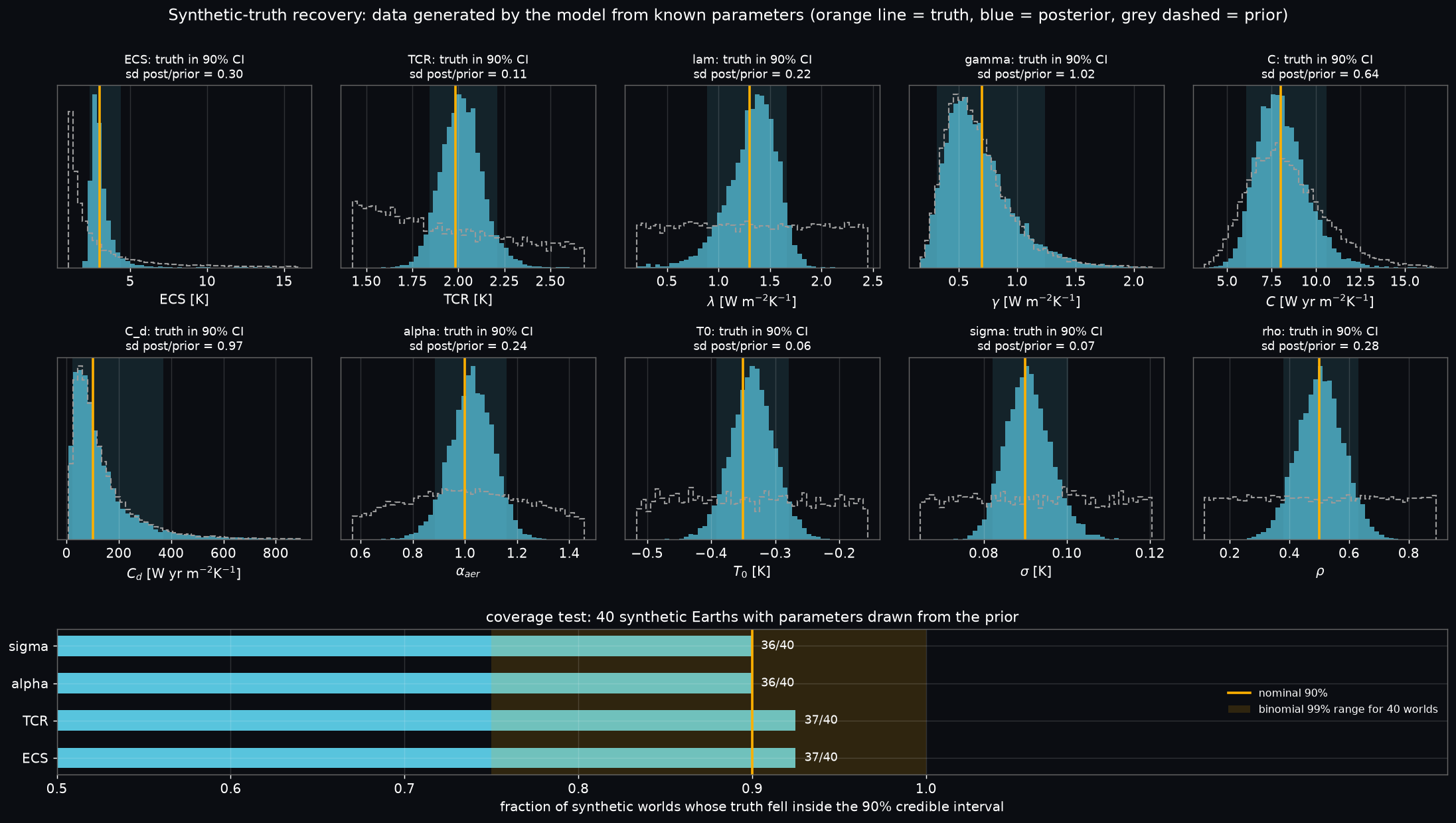
synthetic

We generate a fake record from the model with known parameters (λ = 1.3 so ECS = 3.02 K, γ = 0.7, C = 8, C_d = 100, α = 1, T0 = −0.35, σ = 0.09, ρ = 0.5), using the same years, forcing and AR(1) noise, then run the identical MCMC.

	ECS	TCR	λ	γ	C	C_d	α	T0	σ	ρ
truth	3.02	1.98	1.30	0.70	8.0	100	1.00	−0.35	0.090	0.50
posterior median	2.90	2.02	1.36	0.62	7.9	94	1.03	−0.34	0.091	0.51
inside 90% CI	✓	✓	✓	✓	✓	✓	✓	✓	✓	✓
sd(post)/sd(prior)	0.30	0.11	0.22	1.02	0.64	0.97	0.24	0.06	0.07	0.28

All 10 truths lie inside their 90% intervals. The last row is the real lesson. TCR is learned well (the posterior is 9× narrower than the prior), ECS moderately (3×), and γ and C_d are not learned at all (ratio ≈ 1): they are "recovered" only because the posterior is the prior. Even when the model is exactly right, the surface record cannot identify deep-ocean heat uptake.

Coverage test (bottom panel). A single recovery can succeed by luck. So we draw 40 truths from the prior, simulate 40 synthetic Earths and run 40 MCMCs (32 walkers × 5 000 steps each). The 90% intervals contain the truth in 37/40 (ECS), 37/40 (TCR), 36/40 (α), 36/40 (σ) of them, against an expected 36 ± 1.9 (binomial 99% range ≥ 30). The inference is calibrated. This is a small-scale version of simulation-based calibration (Talts et al. 2018).

ECS and TCR vs IPCC AR6

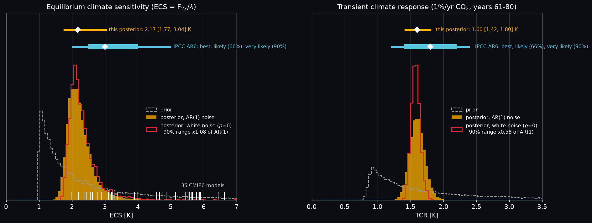
ecs tcr

	This posterior: median, 66%, 90%	IPCC AR6: best, likely (66%), very likely (90%)
ECS	2.17 K, [1.91, 2.56], [1.77, 3.04]	3.0 K, [2.5, 4.0], [2.0, 5.0]
TCR	1.60 K, [1.50, 1.71], [1.42, 1.80]	1.8 K, [1.4, 2.2], [1.2, 2.4]

TCR agrees with AR6: 96% of the posterior lies inside AR6's likely range. The historical record constrains TCR well, because TCR is the historical-type experiment.
ECS is low: P(ECS < 2 K) = 0.28, P(2.5 ≤ ECS ≤ 4) = 0.19, P(ECS > 4) = 0.009. This is a known result, not a new finding. Historical warming has occurred with a sea-surface-temperature pattern that radiates heat away efficiently. As the pattern evolves, feedbacks weaken, so the effective λ seen so far is larger than the long-term λ (the pattern effect; Armour 2017; AR6 Ch. 7, sections 7.4.4 and 7.5.2). A constant-λ model cannot represent this, so it turns an effective sensitivity into ECS. AR6 corrects historical estimates upward for this effect and combines them with process and paleoclimate evidence. Our number is a historical-record-only effective sensitivity with no such correction.
The ECS tail is set by the priors, not the data. While developing this level, two summary rows (Mean, StDev) in the CMIP6 table were accidentally read as models, which made the priors on γ, C and C_d wider. That run gave ECS 2.28 [1.81, 3.51] K but TCR 1.61 [1.42, 1.81] K. The priors moved the ECS 95th percentile by 0.5 K and TCR by 0.01 K. The white ticks are the 35 CMIP6 models' ECS (1.98 to 6.63 K); 26 of them lie above our 95th percentile.

Global sensitivity: Sobol vs one-at-a-time

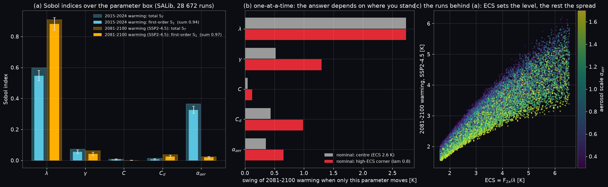
sobol

Inputs are λ ∈ [0.6, 2.4] (ECS 1.6 to 6.6 K), γ ∈ [0.3, 1.2], C ∈ [5, 12], C_d ∈ [40, 200] and α ∈ [0.3, 1.7], treated as independent uniforms. SALib Saltelli sampling uses N = 4096, giving 4096 × (5+2) = 28 672 model runs (about a second with Numba, including the bootstrap confidence intervals).

Output	S₁: λ	γ	C	C_d	α	S_T: λ	γ	C	C_d	α	Σ S₁
2015-2024 warming	0.547	0.056	0.006	0.007	0.327	0.598	0.073	0.008	0.013	0.365	0.943
2081-2100 warming, SSP2-4.5	0.881	0.042	0.000	0.025	0.020	0.908	0.062	0.001	0.037	0.024	0.968

The past and the future care about different things. Today's warming depends on feedback and aerosols (S₁ = 0.55 and 0.33). 2100's depends almost only on feedback (0.88), because aerosol emissions fall in every SSP. This is the structural reason ECS is hard to pin down from history: the parameter that matters for the future shares the historical signal with one that won't.
Interactions are small but real: Σ S₁ = 0.94 and 0.97, so 3 to 6% of the variance comes only from parameter combinations. S_T − S₁ is largest for λ and α in today's warming (0.05 and 0.04).
One-at-a-time (panel b) sweeps each parameter over its range with the others frozen. At the box centre (ECS 2.6 K) the swings in 2100 warming are λ 2.73, γ 0.52, C_d 0.43, α 0.35, C 0.04 K, the same ranking as Sobol. Freeze the others at a high-sensitivity point (λ = 0.8) instead and the swings of γ, C_d and α grow 2.5×, 2.3× and 1.9× (1.30, 0.98, 0.66 K). OAT reports the local slope at whatever point you froze, and explores only 5 lines through a 5-D box. Sobol averages over the whole box and reports how much variance is left unexplained by main effects. Here OAT happens to get the ranking right, but not the magnitudes.
Caveat: Sobol indices describe the box you chose. They assume independent inputs. The posterior is strongly correlated (the ridges above), so a posterior variance decomposition needs Shapley effects or dependent-input methods (OpenTURNS).

Projections: the fan chart, and what it can't say

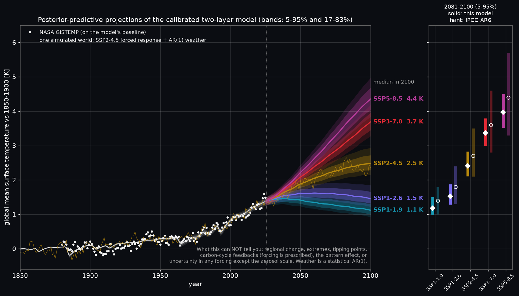
projections

Warming 2081-2100 relative to 1850-1900 (median [5 %, 95 %]), 3 000 posterior draws per scenario:

Scenario	This model	IPCC AR6 (SPM Table SPM.1)
SSP1-1.9	1.18 [0.99, 1.51]	1.4 [1.0, 1.8]
SSP1-2.6	1.52 [1.29, 1.88]	1.8 [1.3, 2.4]
SSP2-4.5	2.42 [2.11, 2.83]	2.7 [2.1, 3.5]
SSP3-7.0	3.37 [3.00, 3.80]	3.6 [2.8, 4.6]
SSP5-8.5	3.97 [3.52, 4.50]	4.4 [3.3, 5.7]

Every median is 0.2 to 0.4 K below AR6 and every range is narrower, especially at the top. Both follow from what the model leaves out:

Low medians come from the low ECS (the pattern effect above). Over this century, projected warming tracks TCR more than ECS, which is why the gap is only 0.2 to 0.4 K.
Narrow ranges come from uncertainty that is simply not in the model: CO₂ and other non-aerosol forcing uncertainty ($F_{2\times}$ alone is ±12%), the pattern effect / state-dependent feedbacks, carbon-cycle feedbacks (the forcing is prescribed), and structural uncertainty. AR6's ranges are built from several lines of evidence and emulators calibrated to all of them.
What this model cannot tell you at all: regional change, extremes, precipitation, sea level, tipping points or abrupt change, anything after 2100 that depends on ice sheets. The thin gold line is "one simulated world" (a posterior draw plus AR(1) weather). The real path will wiggle like that around the fan, with record years and pauses.

So the honest headline is: given this model structure and these priors, the historical record implies roughly the AR6 central warming, somewhat lower, with an uncertainty range we know to be too narrow.

7. Run it

# from SimulationLab/
uv run python L07_earths_thermostat/sim.py

Runtime: 232 s (≈ 4 min wall-clock with uv start-up) on the 8-core dev machine while other agents were running, using 3 Numba threads. Measured breakdown from the section timestamps the script prints: main MCMC 23 s (1.9 M walker-steps), white-noise MCMC 8 s, synthetic recovery 9 s, coverage test 122 s (40 MCMCs, ~3 s each), static figures 14 s, Sobol + OAT ~1 s (28 672 + 210 model runs), projections < 1 s, MP4 51 s. The first run also downloads 1.3 MB (9 files) into data/. Delete a file there to refresh it; otherwise reruns are offline. Everything is seeded (SEED = 2021), and the numbers above reproduce exactly (only the section timings vary).

Outputs in output/: hero.png, projections.png, data_and_forcing.png, mcmc_diagnostics.png, corner.png, posterior_predictive.png, synthetic_truth.png, ecs_tcr_vs_ar6.png, sobol_vs_oat.png, mcmc_walkers.mp4, posterior_summary.csv. The script ends with a PASS/FAIL/REPORT table and raises AssertionError if any check fails:

Check	Expected	Got
AR6 CO₂ ERF = k ln(C/C₀) on Mauna Loa CO₂	R² > 0.99	R² = 0.99985	PASS
implied F₂ₓ = k ln 2 vs AR6 [3.46, 4.40]	inside	3.81 W m⁻²	PASS
exact integrator vs `scipy.linalg.expm` (abrupt 4×CO₂, 5000 yr)	< 1e-9 K	4.4e-14 K	PASS
equilibrium after 5000 yr, T / (F/λ)	1 ± 1e-4	1.000000	PASS
SALib Sobol on Ishigami vs analytic S₁, S_T	< 0.02	0.0023	PASS
emcee: no stuck walkers (acceptance of every walker)	> 0.05	min 0.113, mean 0.131	PASS
chain length after burn-in / τ_max	> 50	113	PASS
no walker parked in a side mode after burn-in	median log-prob gap < 5	0.43	PASS
GISTEMP inside the 90% posterior predictive band	0.80 to 0.98	0.932	PASS
energy imbalance 2006-2018 median vs AR6 [0.52, 1.06] (out of sample)	inside	0.76 W m⁻²	PASS
forced warming 2011-2020 vs AR6 [0.95, 1.20]	inside	1.17 K	PASS
synthetic truth inside 90% CI (10 quantities)	≥ 8 of 10	10 of 10	PASS
synthetic truth inside 99% CI	10 of 10	10 of 10	PASS
90% CI coverage over 40 prior-drawn worlds (ECS, TCR, α, σ)	≥ 30/40 each	37/37/36/36	PASS
TCR median inside AR6 very likely [1.2, 2.4]	inside	1.60 K	PASS
(reported) white-noise likelihood, TCR 90% range	narrower	×0.58	REPORT
(reported) whitened residuals, max \|ACF\| lags 1-10	< 0.16	0.25 at lag 4	miss (ENSO)
(reported) ECS median inside AR6 likely [2.5, 4.0]	inside	2.17 K	miss (pattern effect)

8. Code tour (`sim.py`)

Function	What it does
`fetch`, `load_data`	cached `requests` download; pandas parsing of GISTEMP (`***` gaps), NOAA (`#` header), IPCC ERF and CMIP6 tables
`groups`, `build_forcing`, `split`	ERF → CO₂ / other / aerosol / natural; Mauna Loa log-law fit and 2020-2025 extension; SSP splicing with a tapered offset; (non-aerosol, aerosol) arrays for the model
`ebm`	the model: Numba `prange` kernel, exact exponential map per parameter set, annual-mean output
`model`, `tcr`, `timescales`	contiguous-array wrapper; 1 %/yr CO₂ experiment; fast/slow mode e-folding times
`cmip6_prior`, `log_prior`, `sample_prior`	CMIP6-informed lognormals; hard prior box; rejection sampler (used for walker starts, prior overlays and coverage truths)
`log_like`, `log_prob`	exact AR(1) Gaussian likelihood; vectorised posterior (only in-prior walkers run the model)
`run_mcmc`, `posterior`	emcee sampler (DE + snooker moves, seeded, optional ρ = 0); burn-in, τ, thinning
`verify_integrator`, `verify_sobol`	closed form vs `scipy.linalg.expm`; SALib vs the analytic Ishigami indices
`posterior_predictive`	replicated records, band coverage, trend and ACF test statistics, whitened residuals, energy imbalance
`synthetic_recovery`, `coverage_test`	known-truth MCMC with contraction ratios; 40 prior-drawn worlds for interval coverage
`sensitivity`, `warming`	SALib Sobol for two outputs; one-at-a-time sweeps at two nominal points
`projections`	3 000 posterior draws × 5 SSPs, rebased to 1850-1900; one noisy "simulated world"
`main`	the pipeline, printed numbers and the PASS/FAIL table
`fig_*`, `make_hero`, `mp4_walkers`, `credible_contours`, `fan`, `spread`	plotting only

9. Simplifications & ceilings

Constant feedback, no efficacy. The biggest structural limit. The pattern effect makes historical-only ECS estimates low (above). Upgrade: a deep-ocean efficacy ε (Geoffroy 2013b; the CMIP6 table already has it), or a time-varying λ.
Forcing uncertainty = one aerosol scale. CO₂, other GHGs, volcanic and solar forcing are taken as exact and $F_{2\times}$ is fixed at 3.93. The IPCC repo ships _pc05/_pc95 forcing files that could become prior draws.
2020-2025 forcing is partly a scenario. CO₂ comes from measurements, but everything else follows SSP2-4.5. That misses the 2020 IMO shipping-sulphur cut, the 2022 Hunga Tonga water vapour, the solar-cycle-25 maximum and any aerosol decline beyond the scenario, all candidates for the 2023-2024 warmth that sits above our band.
SSP splice (marked ponytail: in the code). The SSPs diverge from 2015, but our 2020-2025 history follows SSP2-4.5, so each scenario is joined to the 2025 state with an offset that tapers linearly to zero by 2050. Per forcing group the offsets reach 0.27 W m⁻² (SSP1-1.9 aerosols); the net offsets are −0.04 to −0.26 W m⁻². 2081-2100 is untouched, but 2025-2050 is approximate. Per-agent harmonisation (as FaIR and aneris do it) is the upgrade.
AR(1) is the whole error model. Internal variability, GISTEMP measurement uncertainty (larger before 1950) and model structural error are one red-noise process. The lag-4 ENSO signal is left over. A Kennedy & O'Hagan discrepancy term or a state-space (Kalman-filter) EBM (Cummins et al. 2020) separates them.
Priors are choices. Uniform λ favours low ECS; the CMIP6 widening factor (×2, marked ponytail: in the code) is a judgement call. We showed that the ECS tail moves by 0.5 K with it.
Coverage with 40 worlds detects gross miscalibration only (it checks 4 quantities at one level). Full SBC rank histograms would need hundreds of MCMCs, which is fine here (each takes ~2.5 s) but was cut to fit the 5-minute budget.
Sobol over an independent box. The indices describe that box, not the correlated posterior.
emcee is not the best sampler for this job. In 8-D with ridges it needs τ ≈ 60 to 180 steps. Gradient-based NUTS would mix faster but needs a differentiable model.

10. Go further

Rebuild it in FaIR. pip install fair (v2), drive it with the same SSP ERF files, and compare its AR6-calibrated ensemble with our posterior. Then calibrate FaIR's 3-layer EBM with this script's emcee setup.
Add ocean heat to the likelihood. Use NOAA NCEI 0-2000 m ocean heat content, or the von Schuckmann et al. (2023) Earth heat inventory, as a second data stream with its own noise model. Measure how much the posteriors of γ and C_d contract, and whether ECS moves.
Add the pattern effect. Give the model efficacy ε with a CMIP6-informed prior, or let λ drift over time. How close does ECS get to AR6's 3 K, and how much wider do the projections become?
Rewrite in PyMC or Stan. Write the time loop as pytensor.scan or a Stan for loop, sample with NUTS, then use ArviZ for R-hat and ESS. Compare effective samples per second with emcee's.
Emulate an expensive model. Pretend each run costs an hour. Fit a Gaussian-process or polynomial-chaos surrogate on 200 runs (UQLab, OpenTURNS or scikit-learn), run Sobol and MCMC on the surrogate, and check against the exact numbers here.

11. References

I. M. Held et al., "Probing the fast and slow components of global warming by returning abruptly to preindustrial forcing," J. Climate 23, 2418 (2010).
O. Geoffroy et al., "Transient climate response in a two-layer energy-balance model. Part I: Analytical solution and parameter calibration using CMIP5 AOGCM experiments," J. Climate 26, 1841 (2013a); "Part II: Representation of the efficacy of deep-ocean heat uptake and validation for CMIP5 AOGCMs," J. Climate 26, 1859 (2013b).
P. Forster et al., "The Earth's energy budget, climate feedbacks, and climate sensitivity," Ch. 7 in Climate Change 2021: The Physical Science Basis (IPCC AR6 WG1, 2021), with data at github.com/IPCC-WG1/Chapter-7 (C. Smith et al.).
IPCC, Summary for Policymakers in Climate Change 2021: The Physical Science Basis (Table SPM.1).
S. C. Sherwood et al., "An assessment of Earth's climate sensitivity using multiple lines of evidence," Rev. Geophys. 58, e2019RG000678 (2020).
K. C. Armour, "Energy budget constraints on climate sensitivity in light of inconstant climate feedbacks," Nature Climate Change 7, 331 (2017).
N. J. L. Lenssen et al., "Improvements in the GISTEMP uncertainty model," J. Geophys. Res. Atmos. 124, 6307 (2019); GISTEMP Team, NASA GISS Surface Temperature Analysis v4.
G. Myhre et al., "New estimates of radiative forcing due to well mixed greenhouse gases," Geophys. Res. Lett. 25, 2715 (1998).
K. Hasselmann, "Stochastic climate models. Part I. Theory," Tellus 28, 473 (1976).
D. P. Cummins, D. B. Stephenson, P. A. Stott, "Optimal estimation of stochastic energy balance model parameters," J. Climate 33, 7909 (2020).
C. J. Smith et al., "FAIR v1.3: a simple emissions-based impulse response and carbon cycle model," Geosci. Model Dev. 11, 2273 (2018); N. J. Leach et al., "FaIRv2.0.0," GMD 14, 3007 (2021).
D. Foreman-Mackey et al., "emcee: The MCMC Hammer," PASP 125, 306 (2013); J. Goodman, J. Weare, "Ensemble samplers with affine invariance," CAMCoS 5, 65 (2010).
C. J. F. ter Braak, J. A. Vrugt, "Differential Evolution Markov Chain with snooker updater and fewer chains," Stat. Comput. 18, 435 (2008).
I. M. Sobol', "Global sensitivity indices for nonlinear mathematical models and their Monte Carlo estimates," Math. Comput. Simul. 55, 271 (2001).
A. Saltelli et al., "Variance based sensitivity analysis of model output. Design and estimator for the total sensitivity index," Comput. Phys. Commun. 181, 259 (2010); A. Saltelli, P. Annoni, "How to avoid a perfunctory sensitivity analysis," Environ. Model. Softw. 25, 1508 (2010).
J. Herman, W. Usher, "SALib: An open-source Python library for sensitivity analysis," JOSS 2, 97 (2017).
T. Ishigami, T. Homma, "An importance quantification technique in uncertainty analysis for computer models," Proc. ISUMA (1990).
S. Talts et al., "Validating Bayesian inference algorithms with simulation-based calibration," arXiv:1804.06788 (2018).
M. C. Kennedy, A. O'Hagan, "Bayesian calibration of computer models," J. R. Stat. Soc. B 63, 425 (2001).
A. Gelman et al., Bayesian Data Analysis, 3rd ed. (CRC, 2013); A. Gelman et al., "Bayesian workflow," arXiv:2011.01808 (2020).

Every output

mcmc_walkers.mp4

posterior_summary.csv 0 KB

Source code

sim.py 1,098 lines

"""
L07 - Earth's Thermostat: Bayesian calibration of a two-layer climate model on real data.

  live data (NASA GISTEMP, NOAA Mauna Loa CO2, IPCC AR6 forcing, cached in data/)
  -> two-layer energy-balance model (Held 2010 / Geoffroy 2013), exact exponential integrator
  -> emcee posterior with an AR(1) noise likelihood -> MCMC diagnostics
  -> posterior predictive checks + out-of-sample energy-imbalance check
  -> synthetic-truth recovery and a coverage test -> ECS / TCR vs IPCC AR6
  -> SALib Sobol indices vs one-at-a-time -> SSP projection fan charts.

Run from the repo root:   uv run python L07_earths_thermostat/sim.py
"""
import os

os.environ.setdefault("NUMBA_NUM_THREADS", "3")  # CPU etiquette: the machine is shared
os.environ.setdefault("OMP_NUM_THREADS", "1")

import time
from pathlib import Path

import emcee
import imageio_ffmpeg
import matplotlib

matplotlib.use("Agg")
import matplotlib.pyplot as plt
import numpy as np
import pandas as pd
import requests
from matplotlib import animation
from matplotlib.colors import LinearSegmentedColormap
from numba import njit, prange
from SALib.analyze import sobol as sobol_analyze
from SALib.sample import sobol as sobol_sample
from SALib.test_functions import Ishigami
from scipy.linalg import expm
from scipy.ndimage import gaussian_filter

HERE = Path(__file__).parent
DATA, OUT = HERE / "data", HERE / "output"
SEED = 2021  # the year IPCC AR6 WG1 came out

GISTEMP_URL = "https://data.giss.nasa.gov/gistemp/tabledata_v4/GLB.Ts+dSST.csv"
CO2_URL = "https://gml.noaa.gov/webdata/ccgg/trends/co2/co2_annmean_mlo.csv"
IPCC = "https://raw.githubusercontent.com/IPCC-WG1/Chapter-7/main/data_output/"
AR6_URL = IPCC + "AR6_ERF_1750-2019.csv"
SSP_URL = IPCC + "SSPs/ERF_{}_1750-2500.csv"
CMIP6_URL = IPCC + "cmip6_twolayer_tuning_params.csv"

# name, colour (validated for CVD on a dark surface; every fan is also direct-labelled)
SCENARIOS = {"ssp119": ("SSP1-1.9", "#1799b5"), "ssp126": ("SSP1-2.6", "#7a6cf0"),
             "ssp245": ("SSP2-4.5", "#b98a0d"), "ssp370": ("SSP3-7.0", "#e02a35"),
             "ssp585": ("SSP5-8.5", "#b83c9c")}
F2X = 3.93  # AR6 effective radiative forcing of doubled CO2 [W m-2] (sec. 7.3.2.1)
CO2_PI = 278.3  # AR6 1750 CO2 [ppm]
# IPCC AR6 assessments: (5%, 17%, best, 83%, 95%) for ECS/TCR [K], (5%, best, 95%) otherwise
AR6_ECS = (2.0, 2.5, 3.0, 4.0, 5.0)
AR6_TCR = (1.2, 1.4, 1.8, 2.2, 2.4)
AR6_2081_2100 = {"ssp119": (1.0, 1.4, 1.8), "ssp126": (1.3, 1.8, 2.4), "ssp245": (2.1, 2.7, 3.5),
                 "ssp370": (2.8, 3.6, 4.6), "ssp585": (3.3, 4.4, 5.7)}  # SPM Table SPM.1
AR6_WARMING_2011_2020 = (0.95, 1.09, 1.20)  # observed GSAT vs 1850-1900 (SPM A.1.2)
AR6_EEI = {(1971, 2018): (0.43, 0.57, 0.72), (2006, 2018): (0.52, 0.79, 1.06)}  # Table 7.1 [W m-2]

NAMES = ["lam", "gamma", "C", "C_d", "alpha", "T0", "sigma", "rho"]
LABELS = [r"$\lambda$ [W m$^{-2}$K$^{-1}$]", r"$\gamma$ [W m$^{-2}$K$^{-1}$]",
          r"$C$ [W yr m$^{-2}$K$^{-1}$]", r"$C_d$ [W yr m$^{-2}$K$^{-1}$]", r"$\alpha_{aer}$",
          r"$T_0$ [K]", r"$\sigma$ [K]", r"$\rho$"]
# hard prior box; inside it: lambda ~ U, gamma/C/C_d ~ lognormal (CMIP6), alpha ~ N(1, 0.35), rest ~ U
LO = np.array([0.2, 0.05, 1.0, 5.0, 0.0, -1.0, 0.01, 0.0])
HI = np.array([4.0, 5.0, 40.0, 1000.0, 3.0, 1.0, 0.3, 0.95])
ALPHA_SD = 0.35  # AR6 aerosol ERF 1750-2019: -1.1 [-1.7, -0.4] W m-2 -> ~35% (1 sigma) on the scale
TRUTH = np.array([1.3, 0.7, 8.0, 100.0, 1.0, -0.35, 0.09, 0.5])  # synthetic Earth, ECS = 3.02 K


# =============================================================================================
# 1. Data: download once, cache in data/, parse with pandas
# =============================================================================================
def fetch(url):
    """Download once, then reuse the cached copy in data/ (delete the file to refresh)."""
    path = DATA / url.rsplit("/", 1)[-1]
    if not path.exists():
        print(f"  downloading {url}")
        r = requests.get(url, timeout=60)
        r.raise_for_status()
        DATA.mkdir(exist_ok=True)
        path.write_bytes(r.content)
    return path


def load_data():
    gis = pd.read_csv(fetch(GISTEMP_URL), skiprows=1, na_values="***")
    gis = gis.set_index("Year")["J-D"].dropna()  # Jan-Dec means, complete years only [K vs 1951-80]
    co2 = pd.read_csv(fetch(CO2_URL), comment="#").set_index("year")["mean"]  # [ppm]
    erf = pd.read_csv(fetch(AR6_URL), index_col="year")
    ssp = {s: pd.read_csv(fetch(SSP_URL.format(s)), index_col="year") for s in SCENARIOS}
    cmip6 = pd.read_csv(fetch(CMIP6_URL), index_col=0).drop(["Mean", "StDev"])  # summary rows, not models
    last = int(min(gis.index[-1], co2.index[-1]))
    return gis.loc[:last], co2, erf, ssp, cmip6, last


def groups(df):
    """ERF table -> the four groups the model and the figures use [W m-2]."""
    aer = df["aerosol-radiation_interactions"] + df["aerosol-cloud_interactions"]
    nat = df["volcanic"] + df["solar"]
    return pd.DataFrame({"co2": df["co2"], "other": df["total"] - df["co2"] - aer - nat,
                         "aer": aer, "nat": nat})


def build_forcing(erf, ssp, co2, last):
    """Historical ERF 1750..last plus one 1750-2100 run per SSP scenario.

    1750-2019: IPCC AR6 assessed ERF. 2020..last: CO2 from the *measured* Mauna Loa record via a
    log law fitted to AR6 (below); every other agent from SSP2-4.5 (a scenario, not an observation).
    After `last` each SSP takes over; the offset at the splice tapers linearly to zero by 2050.
    """
    hist = groups(erf)
    both = co2.index.intersection(hist.index)
    x, y = np.log(co2[both] / CO2_PI).to_numpy(), hist["co2"][both].to_numpy()
    k = (x @ y) / (x @ x)  # least squares through the origin: F_co2 = k ln(C / C_1750)
    r2 = 1 - ((y - k * x) ** 2).sum() / ((y - y.mean()) ** 2).sum()
    ext = groups(ssp["ssp245"]).loc[2020:last].copy()
    ext["co2"] = hist["co2"][2019] + k * np.log(co2.loc[2020:last] / co2[2019])
    hist = pd.concat([hist, ext])
    runs = {}
    for s in SCENARIOS:
        g = groups(ssp[s])
        fut = g.loc[last + 1:2100]
        # ponytail: linear taper of the seam offset (up to 0.27 W m-2 per group), per-agent
        # harmonisation of the SSP pathways (as FaIR/aneris do) if the 2025-2050 detail matters
        w = np.clip((2050 - fut.index.to_numpy()) / (2050 - last), 0, 1)
        runs[s] = pd.concat([hist, fut + np.outer(w, hist.loc[last] - g.loc[last])])
    return hist, runs, dict(k=k, r2=r2, x=x, y=y, years=both.to_numpy(), ext=ext,
                            ssp245_co2=groups(ssp["ssp245"])["co2"].loc[2020:last])


def split(F):
    """Forcing frame -> (non-aerosol, aerosol) arrays, the two inputs of the model."""
    return (F.sum(axis=1) - F["aer"]).to_numpy(), F["aer"].to_numpy()


# =============================================================================================
# 2. The model: two-layer energy balance, integrated exactly
# =============================================================================================
@njit(parallel=True, fastmath=False, cache=False)
def ebm(theta, fna, fa):
    """Two-layer energy-balance model, one parameter set per row of theta, annual forcing.

        C   dT/dt   = F - lam T - gam (T - T_d)        (mixed layer + atmosphere)
        C_d dT_d/dt =             gam (T - T_d)        (deep ocean)
        F = fna + alpha * fa                           (aerosol ERF scaled by alpha)

    The system is linear, x' = A x + B F, so with F held constant over each year the exact
    one-year map is x_{n+1} = Phi x_n + G F_n with Phi = exp(A) (Sylvester's formula for a 2x2
    with real distinct eigenvalues m1, m2) and G = A^-1 (Phi - I) B. No time-step error at all.
    Returns annual-mean surface temperature (mean of the start/end-of-year states) [K].
    """
    n, nt = theta.shape[0], fna.shape[0]
    out = np.empty((n, nt))
    for i in prange(n):
        lam, gam, C, Cd, alpha = theta[i, 0], theta[i, 1], theta[i, 2], theta[i, 3], theta[i, 4]
        a, b, c, d = -(lam + gam) / C, gam / C, gam / Cd, -gam / Cd  # A = [[a, b], [c, d]]
        det = a * d - b * c  # = lam gam / (C C_d) > 0
        h = np.sqrt(0.25 * (a + d) ** 2 - det)
        m1, m2 = 0.5 * (a + d) + h, 0.5 * (a + d) - h  # slow and fast mode rates (< 0)
        e1, e2 = np.exp(m1), np.exp(m2)
        p00 = (e1 * (a - m2) - e2 * (a - m1)) / (m1 - m2)
        p01 = b * (e1 - e2) / (m1 - m2)
        p10 = c * (e1 - e2) / (m1 - m2)
        p11 = (e1 * (d - m2) - e2 * (d - m1)) / (m1 - m2)
        q0, q1 = (p00 - 1.0) / C, p10 / C  # (Phi - I) B
        g0, g1 = (d * q0 - b * q1) / det, (-c * q0 + a * q1) / det  # A^-1 (Phi - I) B
        T, Td = 0.0, 0.0  # pre-industrial (1750) equilibrium
        for t in range(nt):
            F = fna[t] + alpha * fa[t]
            Tn = p00 * T + p01 * Td + g0 * F
            Td = p10 * T + p11 * Td + g1 * F
            out[i, t] = 0.5 * (T + Tn)
            T = Tn
    return out


def model(theta, fna, fa):
    return ebm(np.ascontiguousarray(np.atleast_2d(theta), dtype=np.float64), fna, fa)


def tcr(theta):
    """Transient climate response: warming around year 70 of a 1 %/yr CO2 ramp (years 61-80)."""
    F = F2X * (np.arange(140) + 0.5) * np.log(1.01) / np.log(2)
    return model(theta, F, np.zeros_like(F))[:, 60:80].mean(1)


def timescales(theta):
    """Fast and slow e-folding times [yr] of the two modes (Geoffroy et al. 2013a)."""
    lam, gam, C, Cd = theta[:, 0], theta[:, 1], theta[:, 2], theta[:, 3]
    tr, det = -(lam + gam) / C - gam / Cd, lam * gam / (C * Cd)
    h = np.sqrt(0.25 * tr**2 - det)
    return -1 / (0.5 * tr - h), -1 / (0.5 * tr + h)


# =============================================================================================
# 3. The Bayesian pieces: prior, AR(1) likelihood, posterior, sampler
# =============================================================================================
def cmip6_prior(cmip6):
    """Lognormal (mu, sd) for gamma, C, C_d from 35 CMIP6 two-layer fits, log-spread doubled.

    ponytail: x2 is a judgement call. A model ensemble shares structural biases, so its spread
    understates real-world uncertainty; doubling lets the data pull outside the model family.
    """
    logs = np.log(cmip6[["gamma_2l", "cmix", "cdeep"]].to_numpy())
    return logs.mean(0), 2.0 * logs.std(0)


def log_prior(th, pri):
    mu, sd = pri
    inside = np.all((th >= LO) & (th < HI), axis=1)
    z = np.log(np.abs(th[:, 1:4]) + 1e-300)  # rows outside the box are masked below
    lp = -(z + 0.5 * ((z - mu) / sd) ** 2).sum(1) - 0.5 * ((th[:, 4] - 1.0) / ALPHA_SD) ** 2
    return np.where(inside, lp, -np.inf)


def sample_prior(n, pri, rng):
    mu, sd = pri
    out = np.empty((0, 8))
    while len(out) < n:  # rejection keeps the draws inside the hard box
        m = 4 * n
        th = np.column_stack([rng.uniform(LO[0], HI[0], m), np.exp(rng.normal(mu, sd, (m, 3))),
                              rng.normal(1.0, ALPHA_SD, m), rng.uniform(LO[5:], HI[5:], (m, 3))])
        out = np.vstack([out, th[np.isfinite(log_prior(th, pri))]])
    return out[:n]


def log_like(th, obs, idx, fna, fa):
    """Exact AR(1) Gaussian likelihood of the residuals r_t = obs_t - (T_model,t + T0).

    r_t = rho r_{t-1} + e_t with e_t ~ N(0, sigma^2), and r_1 drawn from the stationary law
    N(0, sigma^2 / (1 - rho^2)). Whitening: e_t = r_t - rho r_{t-1} must look like white noise.
    """
    r = obs - (model(th, fna, fa)[:, idx] + th[:, 5:6])
    s, rho = th[:, 6], th[:, 7]
    e = r[:, 1:] - rho[:, None] * r[:, :-1]
    n = r.shape[1]
    return (-0.5 * ((e**2).sum(1) + (1 - rho**2) * r[:, 0] ** 2) / s**2 - n * np.log(s)
            + 0.5 * np.log(1 - rho**2) - 0.5 * n * np.log(2 * np.pi))


def log_prob(th, obs, idx, fna, fa, pri):
    """Vectorised over walkers: th is (walkers, 8). Only walkers inside the prior run the model."""
    lp = log_prior(th, pri)
    ok = np.isfinite(lp)
    if ok.any():
        lp[ok] += log_like(th[ok], obs, idx, fna, fa)
    return lp


def run_mcmc(obs, idx, fna, fa, pri, nsteps, nwalkers=48, seed=SEED, white=False):
    """emcee ensemble sampler, walkers started from prior draws (over-dispersed on purpose).

    white=True fixes rho = 0 (i.e. pretends the residuals are independent) for comparison.
    """
    rng = np.random.default_rng(seed)
    p0 = sample_prior(nwalkers, pri, rng)

    def lp(th):
        if white:
            th = np.column_stack([th, np.zeros(len(th))])
        return log_prob(th, obs, idx, fna, fa, pri)

    ndim = 7 if white else 8
    moves = [(emcee.moves.DEMove(), 0.8), (emcee.moves.DESnookerMove(), 0.2)]  # emcee docs' mix
    sampler = emcee.EnsembleSampler(nwalkers, ndim, lp, vectorize=True, moves=moves)
    sampler.random_state = np.random.RandomState(seed).get_state()  # reproducible
    sampler.run_mcmc(p0[:, :ndim], nsteps, progress=False)
    return sampler


def posterior(sampler, burn, white=False):
    """Flat posterior after burn-in, thinned by ~tau/2; rho = 0 column added for white runs."""
    tau = sampler.get_autocorr_time(discard=burn, tol=0)
    flat = sampler.get_chain(discard=burn, thin=max(1, int(tau.max() / 2)), flat=True)
    if white:
        flat = np.column_stack([flat, np.zeros(len(flat))])
    return flat, tau


def ci(x, q=(5, 50, 95)):
    return np.percentile(x, q)


def ar1_noise(sig, rho, n, rng):
    e = np.empty((len(sig), n))
    e[:, 0] = rng.normal(0, sig / np.sqrt(1 - rho**2))
    for t in range(1, n):
        e[:, t] = rho * e[:, t - 1] + rng.normal(0, sig)
    return e


# =============================================================================================
# 4. Verification
# =============================================================================================
def verify_integrator():
    """Our closed-form exponential map vs scipy.linalg.expm for an abrupt-4xCO2 step."""
    th = np.array([[1.3, 0.7, 8.0, 100.0, 1.0]])
    lam, gam, C, Cd = th[0, :4]
    A = np.array([[-(lam + gam) / C, gam / C], [gam / Cd, -gam / Cd]])
    B = np.array([1 / C, 0.0])
    F = 2 * F2X
    nt = 5000
    T_num = model(th, np.full(nt, F), np.zeros(nt))[0]
    x = np.array([np.linalg.solve(A, (expm(A * t) - np.eye(2)) @ B * F)[0] for t in range(nt + 1)])
    err = np.abs(T_num - 0.5 * (x[:-1] + x[1:])).max()
    eq = T_num[-1] / (F / lam)  # after 5000 yr the slow mode (~a few hundred yr) is gone
    return err, eq


def verify_sobol():
    """SALib Sobol on the Ishigami function (a=7, b=0.1) vs its analytic indices."""
    prob = {"num_vars": 3, "names": ["x1", "x2", "x3"], "bounds": [[-np.pi, np.pi]] * 3}
    X = sobol_sample.sample(prob, 8192, calc_second_order=False, seed=SEED)
    Si = sobol_analyze.analyze(prob, Ishigami.evaluate(X), calc_second_order=False, seed=SEED)
    exact_s1, exact_st = np.array([0.3139, 0.4424, 0.0]), np.array([0.5576, 0.4424, 0.2437])
    return max(np.abs(Si["S1"] - exact_s1).max(), np.abs(Si["ST"] - exact_st).max())


# =============================================================================================
# 5. Main pipeline
# =============================================================================================
def main():
    t_start = time.time()
    OUT.mkdir(exist_ok=True)
    plt.style.use("dark_background")
    plt.rcParams.update({"font.size": 11, "axes.grid": True, "grid.alpha": 0.15, "axes.titlesize": 12,
                         "figure.facecolor": "#0b0d12", "axes.facecolor": "#0b0d12",
                         "savefig.facecolor": "#0b0d12", "axes.edgecolor": "#666",
                         "legend.frameon": False})
    rng = np.random.default_rng(SEED)
    checks = []  # (name, expected, got, pass)

    print(f"[{time.time() - t_start:4.0f} s] == 1. data")
    gis, co2, erf, ssp, cmip6, last = load_data()
    hist, runs, co2fit = build_forcing(erf, ssp, co2, last)
    years = hist.index.to_numpy()
    fna, fa = split(hist)
    idx = (gis.index.to_numpy() - 1750).astype(int)
    obs = gis.to_numpy()
    pri = cmip6_prior(cmip6)
    print(f"  GISTEMP {gis.index[0]}-{last} ({len(obs)} yr), Mauna Loa CO2 {co2.index[0]}-{co2.index[-1]}, "
          f"AR6 ERF 1750-2019 + extension to {last}")
    f2x_fit = co2fit["k"] * np.log(2)
    print(f"  CO2 log law fitted to AR6 with Mauna Loa: k = {co2fit['k']:.3f} W/m2, R2 = {co2fit['r2']:.5f}, "
          f"implied F2x = {f2x_fit:.2f} W/m2")
    d_co2 = (co2fit["ext"]["co2"] - co2fit["ssp245_co2"]).to_numpy()
    print(f"  measured-CO2 ERF minus SSP2-4.5 CO2 ERF, 2020-{last}: {d_co2.min():+.3f} .. {d_co2.max():+.3f} W/m2")
    checks.append(("AR6 CO2 ERF = k ln(C/C0) on Mauna Loa CO2", "R2 > 0.99", f"R2 = {co2fit['r2']:.4f}",
                   co2fit["r2"] > 0.99))
    checks.append(("implied F2x = k ln 2 vs AR6 3.93 [3.46, 4.40]", "inside", f"{f2x_fit:.2f} W/m2",
                   3.46 <= f2x_fit <= 4.40))
    fig_data(hist, co2, co2fit, gis, last)

    print(f"[{time.time() - t_start:4.0f} s] == 2. verification of the tools")
    err, eq = verify_integrator()
    print(f"  exact integrator vs scipy expm (abrupt 4xCO2, 5000 yr): max error {err:.2e} K, T/T_eq = {eq:.6f}")
    checks.append(("two-layer integrator vs scipy.linalg.expm", "< 1e-9 K", f"{err:.1e} K", err < 1e-9))
    checks.append(("equilibrium after 5000 yr: T / (F/lam)", "1 +- 1e-4", f"{eq:.6f}", abs(eq - 1) < 1e-4))
    s_err = verify_sobol()
    print(f"  SALib Sobol on Ishigami: max |S - exact| = {s_err:.4f}")
    checks.append(("SALib Sobol S1/ST on Ishigami vs analytic", "< 0.02", f"{s_err:.4f}", s_err < 0.02))

    print(f"[{time.time() - t_start:4.0f} s] == 3. MCMC on the real record")
    t0 = time.time()
    NSTEP, BURN = 30000, 10000  # one walker sat in a spurious high-rho mode until step ~7400
    samp = run_mcmc(obs, idx, fna, fa, pri, NSTEP, nwalkers=64)
    post, tau = posterior(samp, BURN)
    acc = samp.acceptance_fraction
    print(f"  64 walkers x {NSTEP} steps in {time.time() - t0:.1f} s; acceptance {acc.mean():.3f} "
          f"[{acc.min():.2f}-{acc.max():.2f}]; tau = " + ", ".join(f"{n} {t:.0f}" for n, t in zip(NAMES, tau)))
    print(f"  kept {len(post)} samples (burn {BURN}, thin {max(1, int(tau.max() / 2))}); "
          f"(N - burn)/tau_max = {(NSTEP - BURN) / tau.max():.0f}")
    checks.append(("emcee acceptance: no stuck walkers", "every walker > 0.05", f"min {acc.min():.3f}, mean {acc.mean():.3f}",
                   acc.min() > 0.05))
    checks.append(("chain length after burn-in / tau_max", "> 50", f"{(NSTEP - BURN) / tau.max():.0f}",
                   (NSTEP - BURN) / tau.max() > 50))
    lp = samp.get_log_prob()
    gap = np.median(lp[BURN:]) - np.median(lp[BURN:], axis=0).min()  # worst walker vs the ensemble
    stuck = [(w, int(np.where(lp[:, w] < np.median(lp, axis=1) - 15)[0].max()))
             for w in range(lp.shape[1]) if (lp[:, w] < np.median(lp, axis=1) - 15)[2000:].sum() > 200]
    print(f"  walkers >15 log-units below the ensemble for >200 steps after step 2000 (walker, last such step): {stuck}")
    checks.append(("no walker parked in a side mode after burn-in", "worst walker median lp gap < 5",
                   f"{gap:.2f}", gap < 5))
    ecs, tc = F2X / post[:, 0], tcr(post)
    t_fast, t_slow = timescales(post)
    for n, lab, x in zip(NAMES + ["ECS", "TCR", "tau_fast", "tau_slow"], NAMES + ["ECS", "TCR", "tau_f", "tau_s"],
                         list(post.T) + [ecs, tc, t_fast, t_slow]):
        lo, md, hi = ci(x)
        print(f"  {lab:>8s}: {md:8.3f}  [5-95%: {lo:8.3f}, {hi:8.3f}]")
    summary = pd.DataFrame({n: ci(x, (5, 17, 50, 83, 95)) for n, x in
                            zip(NAMES + ["ECS", "TCR"], list(post.T) + [ecs, tc])},
                           index=["p05", "p17", "p50", "p83", "p95"]).T
    summary.to_csv(OUT / "posterior_summary.csv", float_format="%.4f")

    print(f"[{time.time() - t_start:4.0f} s] == 4. white-noise likelihood (rho = 0) for comparison")
    samp_w = run_mcmc(obs, idx, fna, fa, pri, 15000, nwalkers=48, white=True)
    post_w, _ = posterior(samp_w, 7000, white=True)
    ecs_w, tc_w = F2X / post_w[:, 0], tcr(post_w)
    for n, a, b in [("ECS", ecs, ecs_w), ("TCR", tc, tc_w), ("alpha", post[:, 4], post_w[:, 4]),
                    ("T0", post[:, 5], post_w[:, 5]), ("C", post[:, 2], post_w[:, 2])]:
        qa, qb = ci(a), ci(b)
        print(f"  {n:>5s}: AR(1) {qa[1]:.3f} [{qa[0]:.3f}, {qa[2]:.3f}]  white {qb[1]:.3f} [{qb[0]:.3f}, "
              f"{qb[2]:.3f}]  width ratio white/AR(1) {(qb[2] - qb[0]) / (qa[2] - qa[0]):.2f}")
    print(f"  white-noise sigma {np.median(post_w[:, 6]):.3f} vs AR(1) innovation sigma {np.median(post[:, 6]):.3f}")
    wr = np.diff(ci(tc_w, (5, 95)))[0] / np.diff(ci(tc, (5, 95)))[0]
    checks.append(("(reported) white-noise likelihood: TCR 90% range vs AR(1)", "narrower (overconfident)",
                   f"x{wr:.2f}", None))

    print(f"[{time.time() - t_start:4.0f} s] == 5. posterior predictive checks")
    ppc = posterior_predictive(post, obs, idx, fna, fa, gis, years, rng)
    print(f"  obs inside 90% predictive band: {ppc['inside']:.3f}; trend 1975-{last} obs {ppc['t_obs']:.3f} "
          f"K/dec, p = {ppc['p_trend']:.2f}; lag-1 ACF obs {ppc['a_obs']:.2f}, p = {ppc['p_acf']:.2f}")
    print(f"  whitened-residual lag-1 ACF {ppc['acf_white'][1]:+.2f} (raw {ppc['acf_raw'][1]:+.2f}); "
          f"Ljung-Box-style max |ACF| lags 1-10 whitened {np.abs(ppc['acf_white'][1:11]).max():.2f}")
    for (a, b), (lo, md, hi) in AR6_EEI.items():
        q = ci(ppc["eei"][(a, b)])
        print(f"  Earth energy imbalance {a}-{b}: posterior {q[1]:.2f} [{q[0]:.2f}, {q[2]:.2f}] W/m2 "
              f"vs AR6 {md} [{lo}, {hi}]")
    checks.append(("obs inside 90% posterior predictive band", "0.80-0.98", f"{ppc['inside']:.3f}",
                   0.80 <= ppc["inside"] <= 0.98))
    worst = np.argmax(np.abs(ppc["acf_white"][1:11])) + 1
    checks.append(("(reported) whitened residuals white: max |ACF| lags 1-10", f"< {1.96 / np.sqrt(ppc['n']):.2f}",
                   f"{np.abs(ppc['acf_white'][worst]):.2f} at lag {worst}", None))
    q = ci(ppc["eei"][(2006, 2018)])
    checks.append(("EEI 2006-2018 median vs AR6 [0.52, 1.06] (out of sample)", "inside", f"{q[1]:.2f} W/m2",
                   0.52 <= q[1] <= 1.06))
    w1120 = ci(ppc["w2011_2020"])
    print(f"  model warming 2011-2020 vs 1850-1900: {w1120[1]:.2f} [{w1120[0]:.2f}, {w1120[2]:.2f}] K "
          f"vs AR6 1.09 [0.95, 1.20]")
    checks.append(("forced warming 2011-2020 vs AR6 1.09 [0.95, 1.20] K", "inside", f"{w1120[1]:.2f} K",
                   0.95 <= w1120[1] <= 1.20))

    print(f"[{time.time() - t_start:4.0f} s] == 6. synthetic-truth recovery")
    syn = synthetic_recovery(idx, fna, fa, pri, rng)
    for n, (lo, md, hi), tv, c in zip(syn["names"], syn["q"], syn["truth"], syn["contraction"]):
        print(f"  {n:>6s}: truth {tv:8.3f}  posterior {md:8.3f} [90%: {lo:8.3f}, {hi:8.3f}]  "
              f"sd(post)/sd(prior) {c:.2f}")
    n_in = int(sum(lo <= tv <= hi for (lo, _, hi), tv in zip(syn["q"], syn["truth"])))
    n_99 = int(sum(lo <= tv <= hi for (lo, hi), tv in zip(syn["q99"], syn["truth"])))
    checks.append(("synthetic truth inside 90% CI (10 quantities)", "~9 of 10", f"{n_in} of 10", n_in >= 8))
    checks.append(("synthetic truth inside 99% CI (10 quantities)", "10 of 10", f"{n_99} of 10", n_99 == 10))
    print(f"[{time.time() - t_start:4.0f} s]    coverage test (40 synthetic worlds)")
    cov = coverage_test(idx, fna, fa, pri)
    K = cov["K"]
    lo_b = int(np.floor(np.percentile(np.random.default_rng(0).binomial(K, 0.9, 100000), 0.5)))
    for n, h in cov["hits"].items():
        print(f"  coverage of 90% CI over {K} prior-drawn truths, {n}: {h}/{K}")
    checks.append((f"90% CI coverage over {K} synthetic worlds (ECS, TCR, alpha, sigma)",
                   f">= {lo_b}/{K} each (binomial 99%)", "/".join(str(h) for h in cov["hits"].values()),
                   all(h >= lo_b for h in cov["hits"].values())))
    fig_synthetic(syn, cov)

    print(f"[{time.time() - t_start:4.0f} s] == 7. ECS / TCR vs IPCC AR6")
    prior_s = sample_prior(20000, pri, rng)
    ecs_p, tcr_p = F2X / prior_s[:, 0], tcr(prior_s)
    q_ecs, q_tcr = ci(ecs, (5, 17, 50, 83, 95)), ci(tc, (5, 17, 50, 83, 95))
    print(f"  ECS posterior {q_ecs[2]:.2f} K, 66%: [{q_ecs[1]:.2f}, {q_ecs[3]:.2f}], 90%: [{q_ecs[0]:.2f}, "
          f"{q_ecs[4]:.2f}]   AR6: 3.0, likely [2.5, 4.0], very likely [2.0, 5.0]")
    print(f"  TCR posterior {q_tcr[2]:.2f} K, 66%: [{q_tcr[1]:.2f}, {q_tcr[3]:.2f}], 90%: [{q_tcr[0]:.2f}, "
          f"{q_tcr[4]:.2f}]   AR6: 1.8, likely [1.4, 2.2], very likely [1.2, 2.4]")
    print(f"  P(ECS < 2) = {np.mean(ecs < 2):.2f}, P(2.5 <= ECS <= 4) = {np.mean((ecs >= 2.5) & (ecs <= 4)):.2f}, "
          f"P(ECS > 4) = {np.mean(ecs > 4):.3f}, P(ECS > 5) = {np.mean(ecs > 5):.3f}; "
          f"P(1.4 <= TCR <= 2.2) = {np.mean((tc >= 1.4) & (tc <= 2.2)):.2f}")
    print(f"  aerosol ERF 2019 = alpha x {hist['aer'][2019]:.2f} = {np.median(post[:, 4]) * hist['aer'][2019]:.2f} "
          f"[{ci(post[:, 4] * hist['aer'][2019])[2]:.2f}, {ci(post[:, 4] * hist['aer'][2019])[0]:.2f}] W/m2 "
          f"(AR6: -1.1 [-1.7, -0.4])")
    checks.append(("TCR median inside AR6 very likely [1.2, 2.4] K", "inside", f"{q_tcr[2]:.2f} K",
                   1.2 <= q_tcr[2] <= 2.4))
    checks.append(("(reported) ECS median inside AR6 likely [2.5, 4.0] K", "inside", f"{q_ecs[2]:.2f} K",
                   None))
    cm_ecs = cmip6["q4x"] / 2 / -cmip6["lamg"]
    print(f"[{time.time() - t_start:4.0f} s]    figures")
    fig_ecs_tcr(ecs, tc, ecs_w, tc_w, ecs_p, tcr_p, cm_ecs)
    fig_mcmc(samp, BURN, tau)
    fig_corner(post, ecs, tc, prior_s, ecs_p, tcr_p)
    fig_ppc(ppc, gis, last)

    print(f"[{time.time() - t_start:4.0f} s] == 8. global sensitivity: Sobol vs one-at-a-time")
    sob = sensitivity(runs["ssp245"], years)
    for out_name, Si in sob["Si"].items():
        print(f"  {out_name}: S1 " + " ".join(f"{n}={v:.3f}" for n, v in zip(NAMES[:5], Si["S1"]))
              + f"; ST " + " ".join(f"{n}={v:.3f}" for n, v in zip(NAMES[:5], Si["ST"]))
              + f"; sum S1 = {Si['S1'].sum():.3f}")
    for nom, sw in sob["oat"].items():
        print(f"  OAT swing of 2081-2100 warming at nominal {nom}: "
              + " ".join(f"{n}={v:.2f}" for n, v in zip(NAMES[:5], sw)) + " K")
    fig_sensitivity(sob)

    print(f"[{time.time() - t_start:4.0f} s] == 9. projections")
    proj = projections(post, runs, obs, idx, rng)
    for s, (name, _) in SCENARIOS.items():
        q = proj["q2100"][s]
        a = AR6_2081_2100[s]
        print(f"  {name} 2081-2100 vs 1850-1900: {q[1]:.2f} [{q[0]:.2f}, {q[2]:.2f}] K   AR6 {a[1]} [{a[0]}, {a[2]}]")
    m = (gis.index >= 2011) & (gis.index <= 2020)
    print(f"  GISTEMP on the model baseline, 2011-2020 mean: {proj['obs_rel'][m].mean():.2f} K (AR6 1.09 [0.95, 1.20]); "
          f"{last}: {proj['obs_rel'][-1]:.2f} K; forced response {last}: {proj['q']['ssp245'][2][proj['years'] == last][0]:.2f} K")
    fig_projections(proj, gis, last)
    make_hero(proj, gis, last)
    print(f"[{time.time() - t_start:4.0f} s]    writing mcmc_walkers.mp4")
    mp4_walkers(samp, post, obs, idx, gis, fna, fa)

    print("\n== verification & validation")
    ok = True
    for name, exp, got, p in checks:
        flag = "REPORT" if p is None else ("PASS" if p else "FAIL")
        ok &= p is not False
        print(f"  [{flag:6s}] {name}: expected {exp}, got {got}")
    print(f"\ntotal runtime {time.time() - t_start:.0f} s")
    assert ok, "some verification checks failed"


# =============================================================================================
# 6. Analyses
# =============================================================================================
def posterior_predictive(post, obs, idx, fna, fa, gis, years, rng, n=3000):
    th = post[rng.choice(len(post), n)]
    T = model(th, fna, fa)
    base = T[:, (years >= 1850) & (years <= 1900)].mean(1)
    mod = T[:, idx] + th[:, 5:6]
    rep = mod + ar1_noise(th[:, 6], th[:, 7], len(idx), rng)  # replicated data sets
    band = np.percentile(rep, [5, 50, 95], axis=0)
    inside = np.mean((obs >= band[0]) & (obs <= band[2]))
    yrs = gis.index.to_numpy()

    def trend(y, a=1975):
        m = yrs >= a
        return np.polyfit(yrs[m], np.atleast_2d(y)[:, m].T, 1)[0] * 10  # K/decade

    def acf1(y):  # lag-1 autocorrelation of the linearly detrended series
        y = np.atleast_2d(y)
        r = y - np.polynomial.polynomial.polyval(yrs, np.polynomial.polynomial.polyfit(yrs, y.T, 3))
        r = r - r.mean(1, keepdims=True)
        return (r[:, 1:] * r[:, :-1]).sum(1) / (r**2).sum(1)

    t_rep, t_obs = trend(rep), trend(obs)[0]
    a_rep, a_obs = acf1(rep), acf1(obs)[0]
    # residual diagnostics at the posterior median
    med = np.median(post, axis=0)
    r = obs - (model(med, fna, fa)[0, idx] + med[5])
    wht = r[1:] - med[7] * r[:-1]

    def acf(x, k=20):
        x = x - x.mean()
        return np.array([1.0] + [(x[j:] * x[:-j]).sum() / (x**2).sum() for j in range(1, k + 1)])

    # Earth's energy imbalance N = F - lam T (not used in the fit: an out-of-sample check)
    F = fna[None, :] + th[:, 4:5] * fa[None, :]
    N = F - th[:, 0:1] * T
    eei = {(a, b): N[:, (years >= a) & (years <= b)].mean(1) for a, b in AR6_EEI}
    w1120 = T[:, (years >= 2011) & (years <= 2020)].mean(1) - base
    return dict(band=band, mod=np.percentile(mod, [5, 50, 95], axis=0), inside=inside, t_rep=t_rep,
                t_obs=t_obs, p_trend=np.mean(t_rep >= t_obs), a_rep=a_rep, a_obs=a_obs,
                p_acf=np.mean(a_rep >= a_obs), acf_raw=acf(r), acf_white=acf(wht), n=len(r),
                eei=eei, w2011_2020=w1120, resid=r)


def synthetic_recovery(idx, fna, fa, pri, rng):
    """Make data from TRUTH (same years, same forcing, AR(1) noise) and check MCMC gets it back."""
    y = model(TRUTH, fna, fa)[0, idx] + TRUTH[5] + ar1_noise(TRUTH[6:7], TRUTH[7:8], len(idx), rng)[0]
    samp = run_mcmc(y, idx, fna, fa, pri, 15000, nwalkers=48, seed=SEED + 1)
    post, _ = posterior(samp, 7000)
    prior = sample_prior(20000, pri, rng)
    cols = lambda p: [F2X / p[:, 0], tcr(p)] + list(p.T)
    pc, pr = cols(post), cols(prior)
    truth = [F2X / TRUTH[0], tcr(TRUTH)[0]] + list(TRUTH)
    return dict(names=["ECS", "TCR"] + NAMES, truth=truth, post=pc, prior=pr, y=y,
                q=[ci(x) for x in pc], q99=[ci(x, (0.5, 99.5)) for x in pc],
                contraction=[x.std() / p.std() for x, p in zip(pc, pr)])


def coverage_test(idx, fna, fa, pri, K=40):
    """Calibration check: truths drawn from the prior; does the 90% CI contain the truth ~90%?"""
    rng = np.random.default_rng(SEED + 7)
    truths = sample_prior(K, pri, rng)
    hits = {"ECS": 0, "TCR": 0, "alpha": 0, "sigma": 0}
    for k, th in enumerate(truths):
        y = model(th, fna, fa)[0, idx] + th[5] + ar1_noise(th[6:7], th[7:8], len(idx), rng)[0]
        post, _ = posterior(run_mcmc(y, idx, fna, fa, pri, 5000, nwalkers=32, seed=SEED + 100 + k), 2000)
        for n, est, tv in [("ECS", F2X / post[:, 0], F2X / th[0]), ("TCR", tcr(post), tcr(th)[0]),
                           ("alpha", post[:, 4], th[4]), ("sigma", post[:, 6], th[6])]:
            lo, hi = ci(est, (5, 95))
            hits[n] += int(lo <= tv <= hi)
    return dict(K=K, hits=hits)


def warming(theta, fna, fa, years, a, b):
    T = model(theta, fna, fa)
    return T[:, (years >= a) & (years <= b)].mean(1) - T[:, (years >= 1850) & (years <= 1900)].mean(1)


SOBOL_BOUNDS = [[0.6, 2.4], [0.3, 1.2], [5.0, 12.0], [40.0, 200.0], [0.3, 1.7]]


def sensitivity(F245, years_hist):
    """Sobol (Saltelli sampling, SALib) vs one-at-a-time for two outputs of the SSP2-4.5 run."""
    fna, fa = split(F245)
    yrs = F245.index.to_numpy()
    prob = {"num_vars": 5, "names": NAMES[:5], "bounds": SOBOL_BOUNDS}
    X = sobol_sample.sample(prob, 4096, calc_second_order=False, seed=SEED)
    outs = {"2015-2024 warming": warming(X, fna, fa, yrs, 2015, 2024),
            "2081-2100 warming (SSP2-4.5)": warming(X, fna, fa, yrs, 2081, 2100)}
    Si = {k: sobol_analyze.analyze(prob, Y, calc_second_order=False, seed=SEED) for k, Y in outs.items()}
    # one-at-a-time: sweep one parameter over its whole range, the others frozen at a nominal point
    lo, hi = np.array(SOBOL_BOUNDS).T
    oat = {}
    for nom_name, nominal in [("centre (ECS 2.6 K)", (lo + hi) / 2),
                              ("high-ECS corner (lam 0.8)", np.r_[0.8, (lo + hi)[1:] / 2])]:
        sw = []
        for i in range(5):
            th = np.tile(nominal, (21, 1))
            th[:, i] = np.linspace(lo[i], hi[i], 21)
            y = warming(th, fna, fa, yrs, 2081, 2100)
            sw.append(y.max() - y.min())
        oat[nom_name] = np.array(sw)
    return dict(Si=Si, oat=oat, X=X, Y=outs)


def projections(post, runs, obs, idx, rng, n=3000):
    th = post[rng.choice(len(post), n)]
    res = dict(q={}, q2100={}, one={})
    for s, F in runs.items():
        fna, fa = split(F)
        yrs = F.index.to_numpy()
        T = model(th, fna, fa)
        base = T[:, (yrs >= 1850) & (yrs <= 1900)].mean(1, keepdims=True)
        T -= base
        m = yrs >= 1850
        res["years"] = yrs[m]
        res["q"][s] = np.percentile(T[:, m], [5, 17, 50, 83, 95], axis=0)
        res["q2100"][s] = ci(T[:, (yrs >= 2081) & (yrs <= 2100)].mean(1))
        if s == "ssp245":  # observations on the model's 1850-1900 baseline (per-sample offset T0 + base)
            res["obs_rel"] = np.median(obs[None, :] - th[:, 5:6] - base, axis=0)
            j = np.argmin(np.abs(np.median(T[:, -1]) - T[:, -1]))  # a median-ish world, plus weather
            res["one"] = T[j, m] + ar1_noise(th[j:j + 1, 6], th[j:j + 1, 7], m.sum(), rng)[0]
    return res


# =============================================================================================
# 7. Figures
# =============================================================================================
C_OBS, C_MOD, C_AR6, C_PRI = "#f2f2f2", "#ffb000", "#58c4dd", "#9a9a9a"


def savefig(fig, name):
    fig.savefig(OUT / name, dpi=130, bbox_inches="tight")
    plt.close(fig)


def fig_data(hist, co2, fit, gis, last):
    fig, ax = plt.subplots(1, 3, figsize=(17, 5), gridspec_kw={"width_ratios": [1.25, 1, 1.25]})
    y = hist.index
    for col, lab, c in [("co2", "CO$_2$", "#e8e8e8"), ("other", "other GHG, O$_3$, land use...", "#b98a0d"),
                        ("aer", "aerosols", "#58c4dd"), ("nat", "volcanic + solar", "#9a9a9a")]:
        ax[0].plot(y, hist[col], color=c, lw=1.4, label=lab)
    ax[0].plot(y, hist.sum(axis=1), color="#e02a35", lw=2.2, label="total")
    ax[0].axvspan(2019.5, last + 0.5, color="#ffffff", alpha=0.12, lw=0)
    ax[0].text(2017, -2.6, f"2020-{last}: measured CO$_2$\n+ SSP2-4.5 others", ha="right", fontsize=8.5,
               color="#bbb")
    ax[0].set(xlim=(1750, last + 2), ylim=(-3.0, 3.6), xlabel="year", ylabel="effective radiative forcing [W m$^{-2}$]",
              title="(a) IPCC AR6 effective radiative forcing (volcanic spikes clipped)")
    ax[0].legend(loc="upper left", fontsize=9)

    sc = ax[1].scatter(fit["x"], fit["y"], c=fit["years"], cmap="viridis", s=22, zorder=3)
    xx = np.linspace(0, fit["x"].max() * 1.05, 50)
    ax[1].plot(xx, fit["k"] * xx, color=C_MOD, lw=1.5,
               label=f"$F = k\\,\\ln(C/278.3)$, k = {fit['k']:.2f}\nR$^2$ = {fit['r2']:.4f}, "
                     f"$k\\ln 2$ = {fit['k'] * np.log(2):.2f} W m$^{{-2}}$")
    ax[1].plot(xx, 5.35 * xx, color=C_PRI, lw=1.2, ls="--", label="Myhre et al. 1998: k = 5.35")
    ax[1].set(xlabel="ln(CO$_2$ / 278.3 ppm), CO$_2$ from Mauna Loa", ylabel="AR6 CO$_2$ ERF [W m$^{-2}$]",
              title="(b) NOAA Mauna Loa CO$_2$ vs AR6 CO$_2$ forcing")
    ax[1].legend(loc="upper left", fontsize=9)
    cb = fig.colorbar(sc, ax=ax[1], pad=0.01)
    cb.set_label("year")

    v = gis.to_numpy()
    cmap = plt.get_cmap("RdBu_r")
    ax[2].bar(gis.index, v, color=cmap(np.clip((v + 0.6) / 2.0, 0, 1)), width=1.0, lw=0)
    ax[2].set(xlabel="year", ylabel="anomaly vs 1951-1980 [K]", xlim=(1878, last + 2),
              title=f"(c) NASA GISTEMP v4 global mean, 1880-{last}")
    fig.tight_layout()
    savefig(fig, "data_and_forcing.png")


def fig_mcmc(samp, burn, tau):
    chain = samp.get_chain()
    nstep = chain.shape[0]
    fig, axs = plt.subplots(3, 3, figsize=(16, 9.5))
    for i, ax in enumerate(axs.flat[:8]):
        ax.plot(chain[:, :, i], color=C_AR6, alpha=0.08, lw=0.5)
        ax.plot(np.median(chain[:, :, i], axis=1), color=C_MOD, lw=1.0)
        ax.axvspan(0, burn, color="#ffffff", alpha=0.07, lw=0)
        ax.set(ylabel=LABELS[i], xlim=(0, nstep))
        ax.set_xticks(np.linspace(0, nstep, 5), [f"{v / 1000:.0f}k" for v in np.linspace(0, nstep, 5)])
        ax.set_title(f"{NAMES[i]}:  $\\tau$ = {tau[i]:.0f} steps", fontsize=10)
        if i == 0:
            ax.set_yscale("log")
            ax.set_yticks([0.2, 0.5, 1, 2, 4], ["0.2", "0.5", "1", "2", "4"])
            ax.minorticks_off()
            ax.text(burn / 2, 3.6, "burn-in", ha="center", va="top", fontsize=9, color="#bbb")
    for ax in axs[2, :2]:
        ax.set_xlabel("step")
    # autocorrelation time estimate vs chain length (the emcee tutorial's convergence plot)
    ax = axs.flat[8]
    Ns = np.unique(np.geomspace(200, nstep - burn, 14).astype(int))
    post = chain[burn:]
    est = np.array([emcee.autocorr.integrated_time(post[:n], tol=0) for n in Ns])
    for i in range(8):
        ax.loglog(Ns, est[:, i], lw=1.2, alpha=0.9, label=NAMES[i])
    ax.loglog(Ns, Ns / 50, "w--", lw=1.2, label=r"$N/50$")
    ax.set(xlabel="steps after burn-in N", ylabel=r"$\hat\tau$ [steps]",
           title=f"autocorrelation time; acceptance {samp.acceptance_fraction.mean():.2f}")
    ax.legend(fontsize=7.5, ncol=3, loc="upper left")
    fig.suptitle(f"emcee: {chain.shape[1]} walkers x {nstep} steps, walkers started from prior draws "
                 "(orange = median walker)", y=1.0)
    fig.tight_layout()
    savefig(fig, "mcmc_diagnostics.png")


def credible_contours(ax, x, y, rx, ry, color):
    H, xe, ye = np.histogram2d(x, y, bins=45, range=[rx, ry])
    H = gaussian_filter(H, 1.0)
    h = np.sort(H.ravel())[::-1]
    c = np.cumsum(h) / h.sum()
    levels = sorted({h[np.searchsorted(c, q)] for q in (0.95, 0.68)}) + [H.max() * 1.01]
    xc, yc = 0.5 * (xe[1:] + xe[:-1]), 0.5 * (ye[1:] + ye[:-1])
    ax.contourf(xc, yc, H.T, levels=levels, colors=[color], alpha=0.35)
    ax.contourf(xc, yc, H.T, levels=levels[1:], colors=[color], alpha=0.55)
    ax.contour(xc, yc, H.T, levels=levels[:-1], colors=[color], linewidths=0.8)


def fig_corner(post, ecs, tc, prior, ecs_p, tcr_p):
    cols = [ecs, tc, post[:, 4], post[:, 1], post[:, 2], post[:, 3]]
    pcols = [ecs_p, tcr_p, prior[:, 4], prior[:, 1], prior[:, 2], prior[:, 3]]
    labs = ["ECS [K]", "TCR [K]", LABELS[4], LABELS[1], LABELS[2], LABELS[3]]
    rngs = [np.percentile(c, [0.5, 99.5]) for c in cols]
    n = len(cols)
    fig, axs = plt.subplots(n, n, figsize=(13, 13))
    for i in range(n):
        for j in range(n):
            ax = axs[i, j]
            if j > i:
                ax.axis("off")
                continue
            if i == j:
                bins = np.linspace(*rngs[i], 50)
                ax.hist(cols[i], bins=bins, density=True, color=C_MOD, alpha=0.8)
                ax.hist(pcols[i], bins=bins, density=True, histtype="step", color=C_PRI, lw=1.2, ls="--")
                q = ci(cols[i])
                ax.set_title(f"{labs[i].split(' [')[0]} = {q[1]:.2f}$^{{+{q[2] - q[1]:.2f}}}_{{-{q[1] - q[0]:.2f}}}$",
                             fontsize=10)
                ax.set_yticks([])
            else:
                credible_contours(ax, cols[j], cols[i], rngs[j], rngs[i], C_MOD)
                r = np.corrcoef(cols[j], cols[i])[0, 1]
                ax.text(0.95, 0.92, f"r = {r:+.2f}", transform=ax.transAxes, ha="right", va="top", fontsize=8.5)
                ax.set_ylim(*rngs[i])
            ax.set_xlim(*rngs[j])
            ax.grid(False)
            if i == n - 1:
                ax.set_xlabel(labs[j])
            else:
                ax.set_xticklabels([])
            if j == 0 and i > 0:
                ax.set_ylabel(labs[i])
            elif j > 0:
                ax.set_yticklabels([])
    r = lambda a, b: np.corrcoef(cols[a], cols[b])[0, 1]
    fig.text(0.6, 0.8, "Posterior (68% and 95% regions)\nOrange: posterior  |  grey dashed: prior\n"
             "Titles: median and 5-95% range\n\n"
             f"Ridge 1 (TCR-aerosol, r = {r(1, 2):+.2f}): stronger aerosol\n"
             "cooling (bigger alpha) must be offset by a\nlarger transient response to fit the record.\n\n"
             f"Ridge 2 (ECS-gamma, r = {r(0, 3):+.2f}): a sensitive climate\n"
             "hides its warming if the deep ocean\nabsorbs heat faster. Same surface record,\ndifferent futures.",
             fontsize=11, va="top")
    fig.tight_layout()
    savefig(fig, "corner.png")


def fig_ppc(ppc, gis, last):
    yrs = gis.index.to_numpy()
    fig, axs = plt.subplots(2, 2, figsize=(15, 9.5))
    ax = axs[0, 0]
    b = ppc["band"]
    ax.fill_between(yrs, b[0], b[2], color=C_AR6, alpha=0.25, lw=0, label="90% posterior predictive (with AR(1) noise)")
    ax.fill_between(yrs, ppc["mod"][0], ppc["mod"][2], color=C_MOD, alpha=0.45, lw=0, label="90% forced response")
    ax.plot(yrs, ppc["mod"][1], color=C_MOD, lw=1.5)
    obs = gis.to_numpy()
    out = (obs < b[0]) | (obs > b[2])
    ax.plot(yrs, obs, "o", color=C_OBS, ms=3.2, label="GISTEMP")
    ax.plot(yrs[out], obs[out], "o", mfc="none", mec="#e02a35", ms=8, mew=1.4, label="outside the 90% band")
    ax.set(xlabel="year", ylabel="anomaly vs 1951-1980 [K]", xlim=(1878, last + 2),
           title=f"(a) posterior predictive check: {ppc['inside'] * 100:.1f}% of years inside the 90% band")
    ax.legend(loc="upper left", fontsize=9)

    ax = axs[0, 1]
    k = np.arange(len(ppc["acf_raw"]))
    ax.bar(k - 0.18, ppc["acf_raw"], width=0.36, color=C_PRI, label="raw residuals $r_t$")
    ax.bar(k + 0.18, ppc["acf_white"], width=0.36, color=C_MOD, label=r"whitened $e_t = r_t - \rho\, r_{t-1}$")
    ax.axhspan(-1.96 / np.sqrt(ppc["n"]), 1.96 / np.sqrt(ppc["n"]), color="#ffffff", alpha=0.12, lw=0,
               label="white-noise 95% band")
    ax.set_xticks(range(1, len(k), 2))
    ax.set(xlabel="lag [yr]", ylabel="autocorrelation", xlim=(0.4, len(k) - 0.4),
           title="(b) residual autocorrelation at the posterior median")
    ax.legend(fontsize=9)

    ax = axs[1, 0]
    for x, xo, p, lab, c, a in [(ppc["t_rep"], ppc["t_obs"], ppc["p_trend"], f"trend 1975-{last} [K/decade]", C_AR6, 0),
                                (ppc["a_rep"], ppc["a_obs"], ppc["p_acf"], "lag-1 autocorrelation (detrended)", C_MOD, 1)]:
        ins = ax.inset_axes([0.0 + 0.53 * a, 0.0, 0.47, 1.0])
        ins.hist(x, bins=50, color=c, alpha=0.8)
        ins.axvline(xo, color=C_OBS, lw=2)
        ins.set(xlabel=lab, yticks=[])
        ins.set_title(f"observed vs replicated: p = {p:.2f}", fontsize=10)
    ax.axis("off")
    ax.set_title("(c) test statistics: GISTEMP (white line) vs 3000 replicated records", pad=24)

    ax = axs[1, 1]
    for k_, ((a, b_), (lo, md, hi)) in enumerate(AR6_EEI.items()):
        x = ppc["eei"][(a, b_)]
        h = np.histogram(x, bins=60, range=(0, 1.6), density=True)
        ax.stairs(h[0] / h[0].max() * 0.8 + k_, h[1], baseline=k_, fill=True, color=[C_MOD, C_AR6][k_], alpha=0.6)
        ax.errorbar(md, k_ + 0.9, xerr=[[md - lo], [hi - md]], fmt="D", color=C_OBS, capsize=4, ms=6)
        ax.text(1.58, k_ + 0.4, f"{a}-{b_}\nmodel {np.median(x):.2f} W m$^{{-2}}$\nAR6 {md} [{lo}, {hi}]",
                ha="right", va="center", fontsize=9.5)
    ax.set(xlim=(0, 1.6), yticks=[], xlabel="Earth energy imbalance N = F - $\\lambda$T [W m$^{-2}$]",
           title="(d) out-of-sample check: planetary heat uptake (not used in the fit)")
    fig.tight_layout()
    savefig(fig, "posterior_predictive.png")


def fig_synthetic(syn, cov):
    fig = plt.figure(figsize=(17, 9.5))
    gs = fig.add_gridspec(3, 5, height_ratios=[1, 1, 0.8])
    labs = ["ECS [K]", "TCR [K]"] + LABELS
    for k in range(10):
        ax = fig.add_subplot(gs[k // 5, k % 5])
        x, p, tv = syn["post"][k], syn["prior"][k], syn["truth"][k]
        a, b = np.percentile(x, [0.2, 99.8])
        a, b = min(a, tv) - 0.4 * (b - a), max(b, tv) + 0.4 * (b - a)
        rngx = (max(a, np.percentile(p, 0.1)), min(b, np.percentile(p, 99.9)))
        bins = np.linspace(*rngx, 50)
        ax.hist(p, bins=bins, density=True, histtype="step", color=C_PRI, ls="--", lw=1.2)
        ax.hist(x, bins=bins, density=True, color=C_AR6, alpha=0.75)
        lo, md, hi = syn["q"][k]
        ax.axvspan(lo, hi, color=C_AR6, alpha=0.12, lw=0)
        ax.axvline(tv, color=C_MOD, lw=2)
        ax.set(xlabel=labs[k], yticks=[])
        inside = "in" if lo <= tv <= hi else "OUT"
        ax.set_title(f"{syn['names'][k]}: truth {inside} 90% CI\nsd post/prior = {syn['contraction'][k]:.2f}",
                     fontsize=10)
    ax = fig.add_subplot(gs[2, :])
    names = list(cov["hits"])
    h = np.array([cov["hits"][n] for n in names]) / cov["K"]
    ax.barh(names, h, color=C_AR6, height=0.55)
    ax.axvline(0.9, color=C_MOD, lw=2, label="nominal 90%")
    lo, hi = np.percentile(np.random.default_rng(0).binomial(cov["K"], 0.9, 100000), [0.5, 99.5]) / cov["K"]
    ax.axvspan(lo, hi, color=C_MOD, alpha=0.15, lw=0, label=f"binomial 99% range for {cov['K']} worlds")
    for i, v in enumerate(h):
        ax.text(v + 0.005, i, f"{cov['hits'][names[i]]}/{cov['K']}", va="center", fontsize=10)
    ax.set(xlim=(0.5, 1.3), xlabel="fraction of synthetic worlds whose truth fell inside the 90% credible interval",
           title=f"coverage test: {cov['K']} synthetic Earths with parameters drawn from the prior")
    ax.set_xticks(np.arange(0.5, 1.01, 0.1))
    ax.legend(loc="center right", fontsize=9)
    fig.suptitle("Synthetic-truth recovery: data generated by the model from known parameters "
                 "(orange line = truth, blue = posterior, grey dashed = prior)", y=1.0)
    fig.tight_layout()
    savefig(fig, "synthetic_truth.png")


def fig_ecs_tcr(ecs, tc, ecs_w, tc_w, ecs_p, tcr_p, cm_ecs):
    fig, axs = plt.subplots(1, 2, figsize=(15, 5.6))
    for ax, x, xw, xp, ar6, name, xmax in [(axs[0], ecs, ecs_w, ecs_p, AR6_ECS, "ECS", 7.0),
                                           (axs[1], tc, tc_w, tcr_p, AR6_TCR, "TCR", 3.5)]:
        bins = np.linspace(0, xmax, 90)
        ax.hist(xp, bins=bins, density=True, histtype="step", color=C_PRI, ls="--", lw=1.3, label="prior")
        ax.hist(x, bins=bins, density=True, color=C_MOD, alpha=0.75, label="posterior, AR(1) noise")
        wr = np.diff(ci(xw, (5, 95)))[0] / np.diff(ci(x, (5, 95)))[0]
        ax.hist(xw, bins=bins, density=True, histtype="step", color="#e02a35", lw=1.6,
                label=f"posterior, white noise ($\\rho$=0)\n  90% range x{wr:.2f} of AR(1)")
        top = ax.get_ylim()[1]
        y0 = top * 1.08
        ax.plot([ar6[0], ar6[4]], [y0, y0], color=C_AR6, lw=3, solid_capstyle="butt")
        ax.plot([ar6[1], ar6[3]], [y0, y0], color=C_AR6, lw=9, solid_capstyle="butt")
        ax.plot(ar6[2], y0, "D", color="white", ms=7)
        ax.text(ar6[4] + 0.08, y0, "IPCC AR6: best, likely (66%), very likely (90%)", va="center",
                fontsize=9, color=C_AR6)
        q = ci(x)
        y1 = top * 1.2
        ax.plot([q[0], q[2]], [y1, y1], color=C_MOD, lw=3)
        ax.plot(q[1], y1, "D", color="white", ms=7)
        ax.text(q[2] + 0.08, y1, f"this posterior: {q[1]:.2f} [{q[0]:.2f}, {q[2]:.2f}] K", va="center",
                fontsize=9, color=C_MOD)
        ax.set(xlim=(0, xmax), ylim=(0, top * 1.32), xlabel=f"{name} [K]", yticks=[],
               title={"ECS": "Equilibrium climate sensitivity (ECS = F$_{2x}$/$\\lambda$)",
                      "TCR": "Transient climate response (1%/yr CO$_2$, years 61-80)"}[name])
        ax.legend(loc="center right", fontsize=9, bbox_to_anchor=(1.0, 0.42))
    axs[0].plot(cm_ecs, np.full(len(cm_ecs), axs[0].get_ylim()[1] * 0.02), "|", color="white", ms=14, mew=1.2)
    axs[0].text(cm_ecs.max(), axs[0].get_ylim()[1] * 0.07, f"{len(cm_ecs)} CMIP6 models", ha="right",
                fontsize=9, color="#ccc")
    fig.tight_layout()
    savefig(fig, "ecs_tcr_vs_ar6.png")


def fig_sensitivity(sob):
    fig, axs = plt.subplots(1, 3, figsize=(18, 5.6), gridspec_kw={"width_ratios": [1.2, 1, 1]})
    ax = axs[0]
    x = np.arange(5)
    for k, (name, Si) in enumerate(sob["Si"].items()):
        c = [C_AR6, C_MOD][k]
        ax.bar(x + (k - 0.5) * 0.4, Si["ST"], width=0.38, color=c, alpha=0.35, edgecolor=c,
               label=f"{name}: total S$_T$")
        ax.bar(x + (k - 0.5) * 0.4, Si["S1"], width=0.24, color=c, yerr=Si["S1_conf"], capsize=3,
               ecolor="#ddd", label=f"{name}: first-order S$_1$  (sum {Si['S1'].sum():.2f})")
    ax.set_xticks(x, [LABELS[i].split(" [")[0] for i in range(5)])
    ax.set(ylabel="Sobol index", title="(a) Sobol indices over the parameter box (SALib, 28 672 runs)")
    ax.legend(fontsize=8.5, loc="upper right")
    ax = axs[1]
    for k, (nom, sw) in enumerate(sob["oat"].items()):
        ax.barh(x + (k - 0.5) * 0.38, sw, height=0.36, color=[C_PRI, "#e02a35"][k], label=f"nominal: {nom}")
    ax.set_yticks(x, [LABELS[i].split(" [")[0] for i in range(5)])
    ax.invert_yaxis()
    ax.set(xlabel="swing of 2081-2100 warming when only this parameter moves [K]",
           title="(b) one-at-a-time: the answer depends on where you stand")
    ax.legend(fontsize=9, loc="lower right")
    ax = axs[2]
    X, Y = sob["X"], sob["Y"]["2081-2100 warming (SSP2-4.5)"]
    sc = ax.scatter(F2X / X[:, 0], Y, c=X[:, 4], s=3, cmap="viridis", alpha=0.6, rasterized=True)
    cb = fig.colorbar(sc, ax=ax, pad=0.01)
    cb.set_label(r"aerosol scale $\alpha_{aer}$")
    ax.set(xlabel="ECS = F$_{2x}$/$\\lambda$ [K]", ylabel="2081-2100 warming, SSP2-4.5 [K]",
           title="(c) the runs behind (a): ECS sets the level, the rest the spread")
    fig.tight_layout()
    savefig(fig, "sobol_vs_oat.png")


def spread(y, gap):
    """Nudge label heights apart so no two are closer than `gap`, keeping their order."""
    order = np.argsort(y)
    ys = np.asarray(y, float)[order]
    for i in range(1, len(ys)):
        ys[i] = max(ys[i], ys[i - 1] + gap)
    out = np.empty_like(ys)
    out[order] = ys
    return out


def fan(ax, yrs, q, color, lw=2.0, a1=0.16, a2=0.32):
    ax.fill_between(yrs, q[0], q[4], color=color, alpha=a1, lw=0)
    ax.fill_between(yrs, q[1], q[3], color=color, alpha=a2, lw=0)
    ax.plot(yrs, q[2], color=color, lw=lw)


def fig_projections(proj, gis, last):
    fig = plt.figure(figsize=(16, 8))
    gs = fig.add_gridspec(1, 3, width_ratios=[4.2, 0.62, 1], wspace=0.02)
    ax = fig.add_subplot(gs[0])
    yrs = proj["years"]
    hist = yrs <= last
    fan(ax, yrs[hist], proj["q"]["ssp245"][:, hist], "#dddddd", lw=1.5, a1=0.12, a2=0.25)
    end = spread([proj["q"][s][2, -1] for s in SCENARIOS], 0.25)
    for (s, (name, c)), yl in zip(SCENARIOS.items(), end):
        fut = yrs >= last
        fan(ax, yrs[fut], proj["q"][s][:, fut], c)
        ax.text(2102, yl, f"{name}  {proj['q'][s][2, -1]:.1f} K", color=c, va="center",
                fontsize=10.5, fontweight="bold")
    ax.text(2102, end.max() + 0.45, "median in 2100", color="#aaa", fontsize=9.5)
    ax.plot(gis.index, proj["obs_rel"], "o", color=C_OBS, ms=3, label="NASA GISTEMP (on the model's baseline)")
    ax.plot(yrs, proj["one"], color="#b98a0d", lw=0.7, alpha=0.8,
            label="one simulated world: SSP2-4.5 forced response + AR(1) weather")
    ax.axvline(last + 0.5, color="#888", lw=0.8, ls=":")
    ax.set(xlim=(1850, 2100), ylim=(-0.6, 6.5), xlabel="year",
           ylabel="global mean surface temperature vs 1850-1900 [K]",
           title="Posterior-predictive projections of the calibrated two-layer model (bands: 5-95% and 17-83%)")
    ax.legend(loc="upper left", fontsize=9.5)
    ax.text(0.99, 0.02, "What this can NOT tell you: regional change, extremes, tipping points,\n"
            "carbon-cycle feedbacks (forcing is prescribed), the pattern effect, or\n"
            "uncertainty in any forcing except the aerosol scale. Weather is a statistical AR(1).",
            transform=ax.transAxes, ha="right", va="bottom", fontsize=9, color="#aaa")
    ax2 = fig.add_subplot(gs[2], sharey=ax)
    for k, (s, (name, c)) in enumerate(SCENARIOS.items()):
        q, a = proj["q2100"][s], AR6_2081_2100[s]
        ax2.plot([k - 0.15] * 2, [q[0], q[2]], color=c, lw=5, solid_capstyle="butt")
        ax2.plot(k - 0.15, q[1], "D", color="white", ms=6)
        ax2.plot([k + 0.15] * 2, [a[0], a[2]], color=c, lw=5, alpha=0.4, solid_capstyle="butt")
        ax2.plot(k + 0.15, a[1], "o", color="white", ms=6, mfc="none")
    ax2.set_xticks(range(5), [n for n, _ in SCENARIOS.values()], rotation=45, fontsize=9)
    ax2.tick_params(labelleft=False)
    ax2.set_title("2081-2100 (5-95%)\nsolid: this model\nfaint: IPCC AR6", fontsize=10)
    fig.savefig(OUT / "projections.png", dpi=130, bbox_inches="tight")
    plt.close(fig)


def make_hero(proj, gis, last):
    fig = plt.figure(figsize=(16, 9), facecolor="#05070b")
    ax = fig.add_axes([0.06, 0.2, 0.8, 0.64], facecolor="#05070b")
    yrs = proj["years"]
    hist = yrs <= last
    fan(ax, yrs[hist], proj["q"]["ssp245"][:, hist], "#dddddd", lw=1.4, a1=0.10, a2=0.22)
    end = spread([proj["q"][s][2, -1] for s in SCENARIOS], 0.55)
    for (s, (name, c)), yl in zip(SCENARIOS.items(), end):
        fut = yrs >= last
        q = proj["q"][s][:, fut]
        for w, a in [(9, 0.06), (5, 0.12)]:  # glow
            ax.plot(yrs[fut], q[2], color=c, lw=w, alpha=a, solid_capstyle="round")
        fan(ax, yrs[fut], q, c, lw=2.2, a1=0.14, a2=0.3)
        ax.text(2102, yl, f"{name}\n{q[2, -1]:.1f} K [{q[0, -1]:.1f}-{q[4, -1]:.1f}]", color=c,
                va="center", fontsize=12, fontweight="bold", linespacing=1.1)
    ax.text(2102, end.max() + 0.6, "2100: median [5-95%]", color="#999", fontsize=10.5)
    ax.plot(gis.index, proj["obs_rel"], "o", color="#ffffff", ms=3.4, alpha=0.95)
    ax.text(1885, 1.55, "NASA GISTEMP\nobservations", color="#ddd", fontsize=11)
    ax.set(xlim=(1850, 2100), ylim=(-0.5, 6.2))
    ax.set_ylabel("warming vs 1850-1900 [K]", color="#ccc", fontsize=12)
    ax.grid(alpha=0.08)
    for sp in ["top", "right"]:
        ax.spines[sp].set_visible(False)
    ax.tick_params(colors="#bbb", labelsize=11)
    fig.text(0.06, 0.93, "EARTH'S THERMOSTAT", fontsize=30, fontweight="bold", color="white")
    fig.text(0.06, 0.885, "A two-layer climate model, calibrated by MCMC on 146 years of NASA temperatures, "
             "projects five IPCC futures", fontsize=14, color="#bbb")
    # warming stripes: observed until `last`, then one simulated SSP2-4.5 world (median-ish + weather)
    sx = fig.add_axes([0.06, 0.08, 0.8, 0.05])
    obs_y = gis.index.to_numpy()
    fut = yrs > last
    vals = np.r_[proj["obs_rel"], proj["one"][fut]]
    cmap = LinearSegmentedColormap.from_list("stripes", ["#08306b", "#4292c6", "#f7f7f7", "#ef3b2c", "#67000d"])
    colour = cmap(np.clip(0.5 + (vals - 0.6) / 4.4, 0, 1))  # white at 0.6 K (1971-2000-ish), darkest at 2.8 K
    sx.bar(np.r_[obs_y, yrs[fut]], np.ones(len(vals)), width=1.0, color=colour, lw=0)
    sx.axvline(last + 0.5, color="black", lw=2)
    sx.set(xlim=(1850, 2100), ylim=(0, 1), yticks=[])
    sx.tick_params(colors="#bbb", labelsize=10)
    for sp in sx.spines.values():
        sp.set_visible(False)
    fig.text(0.06, 0.14, f"observed 1880-{last}", fontsize=10, color="#bbb")
    fig.text(0.86, 0.14, "one simulated SSP2-4.5 future", fontsize=10, color="#bbb", ha="right")
    fig.text(0.06, 0.02, "Bands: 5-95% and 17-83% posterior (emcee). Forcing: IPCC AR6 ERF + SSPs. Not included: "
             "carbon-cycle feedbacks, pattern effect, non-aerosol forcing uncertainty, regional detail.",
             fontsize=10, color="#888")
    fig.savefig(OUT / "hero.png", dpi=120, facecolor=fig.get_facecolor())
    plt.close(fig)


def mp4_walkers(samp, post, obs, idx, gis, fna, fa):
    """emcee in motion: walkers climb from the prior onto the posterior ridge."""
    plt.rcParams["animation.ffmpeg_path"] = imageio_ffmpeg.get_ffmpeg_exe()
    chain = samp.get_chain()
    steps = np.unique(np.r_[np.arange(40), np.geomspace(40, 3000, 110)].astype(int))
    steps = np.r_[steps, [steps[-1]] * 36]  # hold the last frame
    fig, (a1, a2) = plt.subplots(1, 2, figsize=(12.8, 6.0), gridspec_kw={"width_ratios": [1, 1.25]})
    a1.set(xscale="log", xlim=(0.9, 22), ylim=(0, 2.6), xlabel="ECS = F$_{2x}$/$\\lambda$ [K]",
           ylabel=r"aerosol scale $\alpha_{aer}$")
    lx = np.log10(F2X / post[:, 0])  # final posterior as a faint target (contours in log-ECS)
    H, xe, ye = np.histogram2d(lx, post[:, 4], bins=40, range=[[0, 1.35], [0, 2.6]])
    H = gaussian_filter(H, 1.0)
    h = np.sort(H.ravel())[::-1]
    lev = [h[np.searchsorted(np.cumsum(h) / h.sum(), q)] for q in (0.95, 0.68)]
    a1.contour(10 ** (0.5 * (xe[1:] + xe[:-1])), 0.5 * (ye[1:] + ye[:-1]), H.T, levels=lev, colors="#ffffff",
               linewidths=0.9, alpha=0.6)
    a1.text(1.25, 0.12, "white: final posterior (68/95%)", color="#ccc", fontsize=9)
    a1.set_xticks([1, 2, 3, 5, 10, 20], ["1", "2", "3", "5", "10", "20"])
    a1.axvspan(AR6_ECS[1], AR6_ECS[3], color=C_AR6, alpha=0.12, lw=0)
    a1.text(3.1, 2.5, "AR6 likely ECS", color=C_AR6, fontsize=9, ha="center", va="top")
    trails = [a1.plot([], [], "o", color=C_MOD, ms=m, alpha=a)[0] for m, a in [(2, 0.15), (3, 0.3), (5, 0.9)]]
    yrs = np.arange(len(fna)) + 1750
    a2.plot(gis.index, obs, "o", color=C_OBS, ms=3, zorder=5)
    lines = a2.plot(yrs, np.zeros((len(yrs), chain.shape[1])), color=C_MOD, lw=0.6, alpha=0.35)
    a2.set(xlim=(1850, gis.index[-1] + 1), ylim=(-1.2, 2.5), xlabel="year",
           ylabel="GISTEMP anomaly vs 1951-1980 [K]")
    title = fig.suptitle("")
    fig.tight_layout()

    def update(f):
        s = steps[f]
        for tr, lag in zip(trails, [10, 4, 0]):
            th = chain[max(s - lag, 0)]
            tr.set_data(F2X / th[:, 0], th[:, 4])
        th = chain[s]
        T = model(th, fna, fa) + th[:, 5:6]
        for ln, y in zip(lines, T):
            ln.set_ydata(y)
        title.set_text(f"emcee walkers exploring the posterior: step {s + 1}  "
                       f"(left: parameter space, right: each walker's simulated climate vs NASA data)")
        return trails + lines

    ani = animation.FuncAnimation(fig, update, frames=len(steps), blit=False)
    ani.save(OUT / "mcmc_walkers.mp4", writer=animation.FFMpegWriter(fps=24, bitrate=2400,
                                                                     extra_args=["-pix_fmt", "yuv420p"]), dpi=100)
    plt.close(fig)


if __name__ == "__main__":
    main()