L08 · Generative Bracket
Tell the computer where the bolts go, where the load comes in and how much titanium you can afford, and let it grow the part. This is what the "generative design" button in Fusion 360, Altair Inspire and Ansys Discovery does underneath: a finite-element solver inside an optimiser that moves material to where it carries load. Here it is in one Python file, on a titanium engine-mount bracket after the GE / GrabCAD 2013 jet-engine bracket challenge. It uses the challenge's four load cases, 8 % of the design box, 45 design iterations and about 3.5 minutes of CPU, and the result is a watertight STL you can send to a 3D printer.
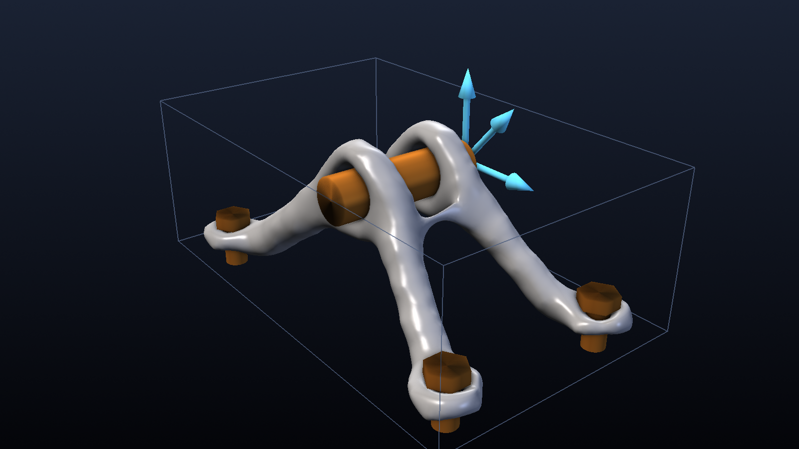
Movies: output/turntable.mp4 (1280×720, 4 s loop) and
output/evolution.mp4 (1280×720, 6.5 s). The second shows the optimiser at work:
the translucent blue cloud is material at density ≥ 0.15, the silver surface is density 0.5, and
the passive lugs and bolt bosses are there from the first frame. Print it:
output/bracket.stl (27,184 triangles, watertight, millimetres).
You are here
Welcome to level 8 of 10. Each level jumps to a new field and adds tools to the stack. This one brings the field every mechanical and aerospace engineer uses daily: finite elements. It also brings the two things that turn FEM into a design tool: sparse iterative solvers that scale to 3D, and gradient-based topology optimisation.
| Level | Field | M&S paradigm | New tools | |
|---|---|---|---|---|
| L01 Wildfire Percolation | Statistical physics / ecology | Cellular automata, Monte Carlo | NumPy, Matplotlib | |
| L02 Noise in Gene Circuits | Synthetic biology | ODEs vs Gillespie SSA | + SciPy | |
| L03 ATL Checkpoint | Operations research | Discrete-event simulation | + SimPy | |
| L04 Echo Chambers | Computational social science | Agent-based models on networks | + Mesa, NetworkX | |
| L05 Galactic Collision | Astrophysics | N-body, HPC Python | + Numba, MP4 | |
| L06 Virtual Wind Tunnel | Fluid dynamics | Lattice Boltzmann CFD, V&V | + Numba stencils | |
| L07 Earth's Thermostat | Climate science | Bayesian calibration, UQ | + pandas, emcee, SALib | |
| ▶ | L08 Generative Bracket | Structural engineering | FEM + 3D topology optimisation | + scikit-fem, pyamg, PyVista/VTK, STL |
| L09 Orbital Traffic Control | Astrodynamics | Real-catalog propagation | + sgp4, Three.js | |
| L10 Solar Stinger | Energy + mobility | Real-data digital twin | + pvlib, GIS |
Things from earlier levels that come back: the "check the fast code against the obviously-correct code" habit (L01), a solver comparison with a scaling plot (L05), and a V&V table with honest misses (L06, L07). Numba (L05) does the one loop NumPy cannot vectorise, and pandas (L07) keeps the tables.
The question
- Design. Take a 176 × 109 × 64 mm design box with four bolts on the bottom and a clevis pin near the top. The pin carries the four GE-challenge load cases: 8,000 lbf up, 8,500 lbf sideways, 9,500 lbf at 42° and 5,000 lbf·in of torsion. Where should 8 % of the box's volume of titanium go to make the stiffest possible bracket, summed over all four cases?
- Trust. Before believing a 3D FE answer, is the solver right? We check a clamped cantilever against Euler–Bernoulli and Timoshenko beam theory at several mesh resolutions, and we check our fast home-made assembly against scikit-fem's reference assembly.
- Cost. Why does every 3D topology optimisation code use an iterative multigrid-preconditioned solver instead of the sparse direct solver that works so well in 2D?
The model
1. Linear elasticity and the FEM pipeline
Small-strain, linear-elastic, isotropic solid (Ti-6Al-4V: $E = 113.8$ GPa, $\nu = 0.342$, 4.43 g/cm³). Units throughout are mm, N and MPa, so compliance comes out in N·mm = mJ.
$$\nabla\cdot\boldsymbol\sigma = \mathbf 0,\qquad \boldsymbol\sigma = \lambda\,\mathrm{tr}(\boldsymbol\varepsilon)\,\mathbf I + 2\mu\,\boldsymbol\varepsilon,\qquad \boldsymbol\varepsilon = \tfrac12(\nabla\mathbf u + \nabla\mathbf u^{\mathsf T}),$$
with $\mathbf u = \mathbf 0$ on the clamped boundary and traction $\mathbf t$ on the loaded boundary. The finite-element method turns this into a linear system in five steps:
| Step | What happens | In the code |
|---|---|---|
| Weak form | Multiply by a test field $\mathbf v$ and integrate by parts: find $\mathbf u$ with $\int_\Omega \boldsymbol\sigma(\mathbf u):\boldsymbol\varepsilon(\mathbf v)\,d\Omega = \int_{\Gamma_t}\mathbf t\cdot\mathbf v\,d\Gamma$ for all admissible $\mathbf v$. Only first derivatives remain, so piecewise-polynomial fields are allowed. | skfem.models.elasticity.linear_elasticity is exactly this bilinear form |
| Element stiffness | On each element $\mathbf u \approx \sum_a N_a \mathbf u_a$ with trilinear shape functions (8 nodes × 3 dofs = 24). Then $\mathbf k_e = \int_{\Omega_e}\mathbf B^{\mathsf T}\mathbf D\,\mathbf B\,d\Omega$, evaluated by 2×2×2 Gauss quadrature ($\mathbf B$ = strain–displacement matrix, $\mathbf D$ = elasticity matrix). | voxel_fem: scikit-fem integrates the form on one voxel; every voxel is a translated copy, so one 24×24 $\mathbf k_0$ serves all |
| Assembly | $\mathbf K = \sum_e \mathbf P_e^{\mathsf T}(E_e\,\mathbf k_0)\,\mathbf P_e$: scatter-add each element matrix into the global sparse matrix via its dof map. | set_supports precomputes where each of the $24^2$ entries lands in the CSR array, and scatter (Numba) adds them: about 0.1 s for 23 M entries |
| Boundary conditions | Dirichlet: delete the rows and columns of fixed dofs (what scikit-fem's condense does). Loads: nodal forces. For a uniform traction on bilinear faces the consistent weights are 1 (interior node), ½ (edge) and ¼ (corner). |
set_supports, bracket, cantilever_voxel |
| Sparse solve | $\mathbf K\mathbf u = \mathbf f$, where $\mathbf K$ is symmetric positive-definite with about 81 non-zeros per row. | solve → amg + pcg |
2. Why AMG-preconditioned CG beats a direct solver in 3D
A sparse direct solver (Cholesky or LU) factorises $\mathbf K$. The factors "fill in": entries
that were zero become non-zero. For a 2D grid the fill is mild. For a 3D grid even the best ordering
(nested dissection, George 1973) must eliminate separator planes of $N^{2/3}$ unknowns, which become
dense blocks. That costs $O(N^{4/3})$ memory and $O(N^{2})$ flops, and it is why "just call
spsolve" dies somewhere past $10^5$ unknowns in 3D.
Conjugate gradients (CG) needs only matrix–vector products ($O(N)$ memory), but its iteration count grows like $\sqrt{\kappa(\mathbf K)}$, and $\kappa \propto h^{-2}$. With a simple diagonal (Jacobi) preconditioner that means $\propto 1/h \propto N^{1/3}$ iterations, so $O(N^{4/3})$ work, and SIMP makes it worse: void regions have a stiffness $10^{9}$ times smaller than solid.
Algebraic multigrid (AMG) fixes the conditioning. CG's slow-to-converge error components are
smooth, low-energy modes. A multigrid V-cycle removes the high-frequency error with a cheap
smoother (Gauss–Seidel) and hands the smooth remainder to a coarser copy of the problem, recursively.
Algebraic means the coarse levels are built from the matrix alone, with no geometry needed.
Smoothed aggregation (Vaněk, Mandel & Brezina 1996) groups nodes into aggregates. For elasticity it
must be told the near-null space, the six rigid-body modes (3 translations and 3 rotations)
that cost no strain energy. rigid_body_modes builds them, and pyamg keeps them exactly
representable on every level. Used as a CG preconditioner, the V-cycle gives an iteration count that
barely depends on $N$ (9–13 here from 2×10³ to 2×10⁵ unknowns), so the total work is $O(N)$.
Topology optimisation adds two more reasons to go iterative. The matrix changes every design iteration,
so a factorisation is never reused. And the previous design's displacement is an excellent initial guess
(warm start), which only an iterative method can exploit.
3. SIMP: from "where is material" to a smooth optimisation problem
Each voxel $e$ gets a density $\rho_e \in [0,1]$ and a Young's modulus (Solid Isotropic Material with Penalisation, Bendsøe 1989):
$$E_e(\tilde\rho_e) = E_{\min} + \tilde\rho_e^{\,p}\,(E_0 - E_{\min}),\qquad p = 3,\ E_{\min} = 10^{-9}E_0 .$$
The optimisation problem, for load cases $k = 1..4$, is
$$\min_{\boldsymbol\rho}\ c = \sum_k \mathbf f_k^{\mathsf T}\mathbf u_k \quad\text{s.t.}\quad \mathbf K(\tilde{\boldsymbol\rho})\,\mathbf u_k = \mathbf f_k,\qquad \frac{1}{N_e}\sum_e \tilde\rho_e = V^* = 0.08,\qquad 0 \le \rho_e \le 1 .$$
Compliance $c$ is the work done by the loads, and minimising it means maximising stiffness. The problem is self-adjoint, so the gradient needs no extra solve:
$$\frac{\partial c}{\partial\tilde\rho_e} = -\,p\,\tilde\rho_e^{\,p-1}(E_0 - E_{\min})\sum_k \mathbf u_{k,e}^{\mathsf T}\mathbf k_0\,\mathbf u_{k,e}.$$
Why penalise? With $p = 1$ stiffness is proportional to density, so half-dense material is exactly as efficient as full material spread thinner. The optimum is a smooth grey "variable-thickness sheet" you cannot manufacture (top panel of the MBB figure below). With $p = 3$ a half-dense voxel costs half the volume but gives only 1/8 of the stiffness. Grey becomes a bad deal, and the optimiser pushes densities to 0 or 1 on its own.
4. The density filter, and why checkerboards happen
Run SIMP on bilinear/trilinear elements without regularisation and you get checkerboards: solid and void voxels alternating like a chessboard (middle panel below). They are a numerical artefact. Two solid elements touching only at a corner node still transfer load through that node, and low-order elements overestimate the stiffness of such a pattern (Díaz & Sigmund 1995). The optimiser is doing its job perfectly and exploiting a flaw in the discretisation. Here the unfiltered design reports a lower compliance (185.4) than the clean one (194.6). A second problem is mesh dependence. Without a length scale the continuum problem wants ever-finer members, so refining the mesh changes the answer instead of converging it.
The density filter (Bruns & Tortorelli 2001, Bourdin 2001) fixes both. The physical density is a weighted average of the design variables within a radius $r_{\min}$:
$$\tilde\rho_e = \frac{\sum_i H_{ei}\,\rho_i}{\sum_i H_{ei}},\qquad H_{ei} = \max\bigl(0,\ r_{\min} - \lVert\mathbf x_e - \mathbf x_i\rVert\bigr).$$
Nothing can vary faster than the filter allows, so checkerboards average out and members are at least
about $2r_{\min}$ wide. The chain rule sends gradients back through the same weights,
$\partial c/\partial\rho_i = \sum_e H_{ei}\,(\partial c/\partial\tilde\rho_e)/\sum_j H_{ej}$. The grid is
regular, so $\mathbf H$ is never stored. It is a 3D correlation with a cone kernel
(scipy.ndimage.correlate), and its adjoint is the same correlation because the kernel is symmetric. The
price is a grey band about one filter radius wide at every surface (23 % "grey" in the bottom MBB panel). We
cut through that band with the $\tilde\rho = 0.5$ isosurface. A Heaviside projection would remove
it (see Go further).
5. The optimality-criteria (OC) update
The KKT condition for a single volume constraint is $B_e \equiv -\dfrac{\partial c/\partial\rho_e}{\lambda\,\partial V/\partial\rho_e} = 1$ wherever $0 < \rho_e < 1$. OC turns this into a fixed-point update (Bendsøe & Sigmund 2003):
$$\rho_e^{\text{new}} = \mathrm{clamp}\Bigl(\rho_e\,B_e^{\,\eta},\ \ \rho_e \pm m,\ \ [0,1]\Bigr),\qquad \eta = \tfrac12,\ m = 0.2 .$$
The Lagrange multiplier $\lambda$ is found by bisection so that the filtered volume hits 8 % exactly after every step. Elements with $B_e > 1$ are doing more than their share of work and grow. The others shrink. OC is a heuristic, but for one constraint it is hard to beat. With several constraints (stress, frequency, several volumes) you switch to MMA (Svanberg 1987), which is what the commercial codes use.
6. The bracket problem
| Item | Value |
|---|---|
| Design box | 176 × 108.8 × 64 mm, voxels of 3.2 mm. The half model ($y \ge 0$) is 55 × 17 × 20 = 18,700 voxels |
| Clevis | pin Ø 19.2 mm along $y$ at $x = 88$, $z = 44$ mm. Two lugs (passive solid, outer R 19.2 mm, 12.8 mm thick, at 11.2 ≤ |y| ≤ 24 mm), a passive-void slot between them for the mating tongue |
| Bolts | four, at $(x, y) = (18, \pm36)$ and $(158, \pm36)$ mm. Passive-solid bosses (R 12.8 mm, 9.6 mm tall) with Ø 9.6 mm holes, and a passive-void column above each boss for bolt-head and wrench access. Supports: boss bottom faces clamped |
| Loads (at the pin bore, spread evenly over the bore nodes) | vertical 8,000 lbf · horizontal ($+x$) 8,500 lbf · 42° from vertical 9,500 lbf · torsion 5,000 lbf·in about the horizontal $x$ axis (the two lugs pushed in opposite $z$ directions) |
| Optimiser | SIMP $p = 3$, $E_{\min} = 10^{-9}E_0$, filter $r_{\min}$ = 1.5 voxels (4.8 mm), OC with move 0.2, $V^* = 0.08$, 45 iterations |
| Linear solver | pyamg smoothed-aggregation AMG + CG, relative residual $10^{-5}$, warm-started from the previous iteration |
Symmetry, including the torsion case. The part is symmetric about $y = 0$, so we mesh half of it. The three force cases are symmetric, so on the mid-plane $u_y = 0$. The torsion case is antisymmetric (mirror the part and the load flips sign), so on the mid-plane $u_x = u_z = 0$ instead. Any load splits into a symmetric and an antisymmetric part, so this decomposition is exact: two sets of supports, two AMG hierarchies, half the unknowns each (61,932 and 60,756). The half model's compliance is half the full part's. All compliances quoted below are for the full part. The per-iteration console log prints the half-model value.
7. The verification problem
A 50 × 10 × 10 mm titanium cantilever ($L/b = 5$, stubby on purpose so that shear matters) is clamped on one end face. It carries a 1 kN uniform shear traction on the other, and we measure the work-conjugate tip deflection $\delta = \mathbf f\cdot\mathbf u/P$ (the traction-weighted mean of $u_z$ over the tip face).
$$\delta_{EB} = \frac{PL^3}{3EI} = 0.4394\ \text{mm},\qquad \delta_{T} = \frac{PL^3}{3EI} + \frac{PL}{\kappa G A} = 0.4532\ \text{mm},\qquad \kappa = \frac{10(1+\nu)}{12+11\nu} = 0.851 \ \text{(Cowper 1966)} .$$
At this aspect ratio shear adds 3.2 % to the deflection.
M&S concepts you'll learn here
- The FEM pipeline: strong form → weak form → shape functions → element matrices → assembly → boundary conditions → sparse linear algebra. Every commercial structural code runs these steps.
- Code verification vs solution verification. The fast voxel code reproduces scikit-fem's generic assembly to 2×10⁻¹³ (code verification). Mesh refinement shows the discretisation error shrinking at the expected rate (solution verification).
- Model-form error is not discretisation error. The fully converged 3D answer is 1.7–2 % stiffer than Timoshenko beam theory. That gap does not close with refinement, because the 3D clamp and beam theory describe slightly different problems.
- Shear locking and p- vs h-refinement. Fully integrated trilinear hexes are far too stiff in bending (15 % too stiff at 2 elements through the thickness, against the converged 3D answer). Triquadratic hexes with the same 297 dofs are 2 % off. This is why Abaqus has C3D8I and C3D20 elements.
- Preconditioning and multigrid. Condition numbers, why Jacobi-CG iterations grow like $N^{1/3}$, what "near-null space" means, and why smoothed aggregation needs the rigid-body modes.
- Adjoint sensitivities. One extra solve (zero, here, because compliance is self-adjoint) gives the gradient with respect to 18,700 design variables at once.
- Regularisation of ill-posed problems. Without the filter the optimum does not exist in the continuum. With it you get a length scale and mesh-independent designs.
- Symmetry reduction for symmetric and antisymmetric load cases, and superposition (linear elasticity: one AMG hierarchy serves every load case on the same supports).
- Multi-load-case design. The objective is a sum of compliances, so the part is a compromise, not a single-load truss.
- From field to geometry: isosurface extraction (marching cubes / flying edges), Taubin smoothing (smoothing without shrinkage), Loop subdivision and a watertight STL. This is the CAD hand-off every generative-design tool has to solve.
Tech stack
| Tool | Since | Role here |
|---|---|---|
| Python 3.12 | L01 | glue |
| NumPy | L01 | voxel-mesh index arithmetic (np.indices), element strain energies and stresses (einsum), the OC bisection |
| Matplotlib | L01 | verification, solver-benchmark, MBB and convergence figures |
| SciPy | L02 | CSR sparse matrices, SuperLU (splu) for 2D and for the direct-solver benchmark, ndimage.correlate as the density filter |
| SimPy, Mesa, NetworkX | L03–L04 | not needed: this is continuum mechanics, not events or agents |
| Numba | L05 | the assembly scatter-add. It is the one loop with data-dependent writes that NumPy can only do with a slower bincount |
| imageio-ffmpeg | L05 | H.264 MP4 (yuv420p). PyVista frames are piped straight into ffmpeg |
| pandas | L07 | verification and benchmark tables, history.csv |
| ★ scikit-fem | L08 | Weak forms written as Python functions, assembled into sparse matrices. It gives us the element stiffness for the optimiser (Hex8 in 3D, Quad4 in 2D), and it is also an independent end-to-end FE pipeline (Hex8 and Hex27, FacetBasis traction, condense) that the fast code is verified against. It is pure NumPy, so it is easy to read, but its generic assembly is slow (a Hex27 mesh with 10k dofs takes about 2 min), which is why the optimiser only borrows $\mathbf k_0$ from it |
| ★ pyamg | L08 | Smoothed-aggregation algebraic multigrid with a user-supplied near-null space (rigid-body modes), plus its CG with residual history. This makes 3D solves $O(N)$ |
| ★ PyVista / VTK | L08 | ImageData voxels → contour (flying-edges marching cubes) → smooth_taubin → Loop subdivide → off-screen rendering with a three-point light rig and SSAO → STL writer. VTK is the engine inside ParaView, and PyVista is its Pythonic front end |
| ★ STL | L08 | a triangle soup with normals, the lingua franca of 3D-print slicers. Ours is closed (no open edges), so it slices as a solid |
Industry & scientific tools
| Tool | What it is | Who uses it | How this project maps to it |
|---|---|---|---|
| Ansys Mechanical (+ Topology Optimization, Ansys Discovery) | General-purpose implicit FE. Its topology-optimisation analysis is a density method with manufacturing constraints. Discovery runs it live on the GPU | aerospace, automotive, energy | Our loop is what its Topology Optimization system runs, on unstructured tets instead of voxels. Its solver switch "Sparse Direct vs PCG" is exactly our LU vs AMG-CG benchmark |
| Abaqus + Tosca Structure (Dassault) | Nonlinear FE, plus Tosca for sensitivity-based (SIMP-like) and condition-based topology optimisation | automotive, aero, medical devices | Tosca's sensitivity-based run is this code plus stress, frequency and manufacturing constraints. Abaqus's C3D8 locks like our Hex8, while C3D8I (incompatible modes) and C3D20 (serendipity, a cousin of our Hex27) are the cures |
| Altair OptiStruct / Inspire | The first commercial topology-optimisation solver (1994), a SIMP density method with member-size, draw-direction, extrusion and symmetry constraints. Inspire is the designer-facing GUI | automotive and aerospace lightweighting | OptiStruct's DTPL + MINDIM = our densities + $r_{\min}$. Its symmetry constraint is our half model |
| nTop (nTopology) | Implicit (field-based) CAD for additive manufacturing | aerospace AM, medical implants, heat exchangers | Takes a density field or STL and makes it printable (smooth, offset, thicken, lattice-fill). Our isosurface + Taubin smoothing is the minimal version of that step |
| Autodesk Fusion 360 Generative Design | Cloud service that runs many optimisations (level-set based) across materials, manufacturing methods and targets, and returns editable geometry | product designers, small manufacturers | "Generative" = this loop run many times with different $V^*$, materials and constraints, followed by B-rep/T-spline reconstruction instead of an STL, and re-analysis of the smoothed part |
| COMSOL Multiphysics (Optimization Module) | Equation-based multiphysics FE. Density-method TO with a Helmholtz PDE filter and MMA | academia, industrial R&D | Our cone filter ≈ its Helmholtz filter. Our OC ≈ its MMA restricted to one constraint |
| FEniCS / dolfinx | Python FE framework: weak forms in UFL, compiled kernels, PETSc solvers, MPI | research | scikit-fem's role here at HPC scale. dolfinx + PETSc GAMG (smoothed aggregation) is the parallel version of our pyamg solve, and dolfin-adjoint automates the sensitivity |
| deal.II | C++ adaptive-FE library (hexahedra, AMG via Trilinos, MPI) | research, large-scale TO | the same pipeline with adaptive meshes and millions of cores |
| PETSc TopOpt (Aage et al.) | Open-source parallel C++ TO framework: SIMP + density filter + MMA + multigrid-preconditioned Krylov | research; the 1.1-billion-voxel aircraft wing (Nature 2017) | literally this algorithm (voxels, SIMP, filter, MG-CG) on 8,000 cores |
| ParaView | VTK GUI for large scientific data | everyone who post-processes simulations | Our contour → smooth_taubin → render chain is four ParaView filters in a script |
What the commercial tools add on top of this script: CAD-conforming unstructured meshes; manufacturing constraints (additive overhang angle, casting draw direction, milling access, minimum and maximum member size, symmetry and patterns); stress, displacement, frequency and buckling constraints; general-purpose optimisers (MMA, SQP); geometry reconstruction from the density field into editable CAD; and, most importantly, re-analysis of the reconstructed part. The smoothed geometry is a new design and has to be verified again with a body-fitted mesh before anyone signs off.
Results
The bracket
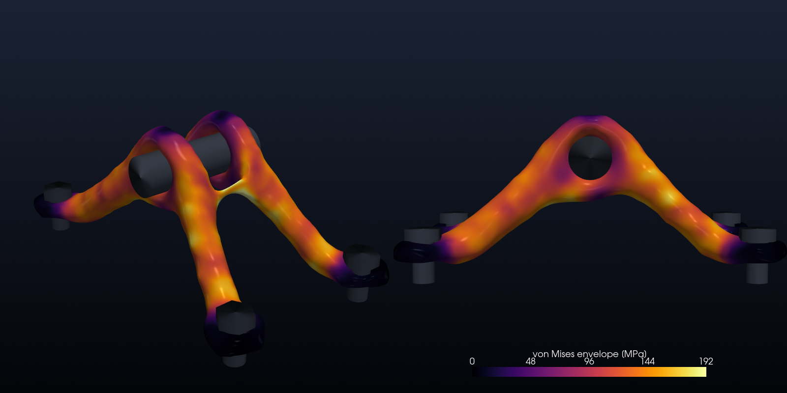
The optimiser found a pair of A-frames. Each lug sends one leg down to each of the two bolts on its side, so the pin sits at the apex of both frames. Three things are worth noticing:
- Nearly uniform stress. Along the legs the von Mises envelope sits at roughly 120–190 MPa. It is low only near the clamped bosses and on the lug crowns. A stiffness optimum ends up close to a fully stressed design, where every member works equally hard (Michell 1904). The envelope on the surface is 192 MPa at the 99th percentile and 221 MPa at its maximum. Against Ti-6Al-4V's yield (about 880 MPa) that is a factor of about 4. These are voxel-resolution stresses on a compliance design, not a certification (see Simplifications).
- Mass. The printable isosurface encloses 79.2 cm³ (6.5 % of the 1,226 cm³ box), or 351 g of Ti-6Al-4V. That is less than the design's 8 % because the grey material below $\tilde\rho = 0.5$ is cut off. For scale, GE's original bracket weighed about 2 kg and the winning challenge entries about 0.33 kg. Their interface geometry, design envelope and stress requirements differ from our simplified version, so treat this as a sanity check, not a comparison.
- Stiffness per mass. Filling the whole design box with titanium (minus the keep-out voids, 90 % of the box) gives a total compliance of 1,694 N·mm. The optimised part gives 14,192 N·mm, i.e. 8.4× more compliant with 11.3× less material, so it has 1.35× the stiffness per unit mass of a solid block. That margin is modest because the sum of four very different load cases forces a compromise. A single-load MBB beam gains far more.
Optimisation history
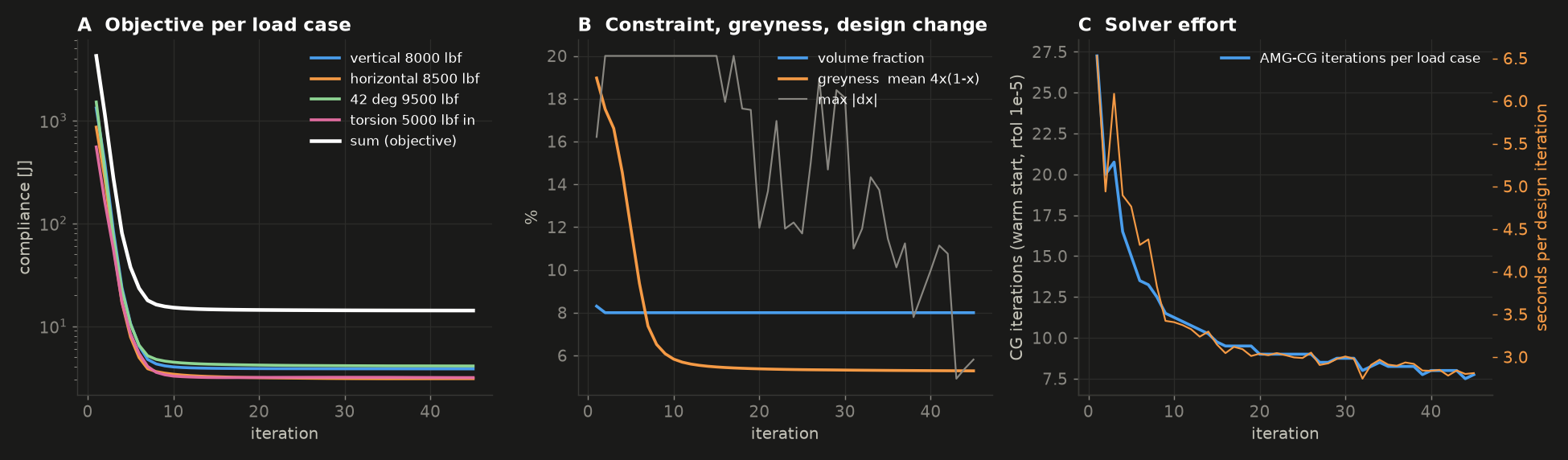
| iteration 1 | 10 | 20 | 45 (final) | |
|---|---|---|---|---|
| total compliance, N·mm | 4,248,137 | 15,163 | 14,377 | 14,192 |
| vertical / horizontal / 42° / torsion | 3,843 / 3,088 / 4,100 / 3,160 | |||
| volume fraction | 0.083 | 0.0800 | 0.0800 | 0.0800 |
| greyness $\overline{4\tilde\rho(1-\tilde\rho)}$ | 19 % | 5.8 % | 5.4 % | 5.3 % |
| AMG-CG iterations per load case | 27 | 11 | 9 | 8 |
The first iterate is a uniform grey cloud that the four loads can barely hold up. Within ten iterations the legs exist, and the last 25 iterations only refine the shape: compliance falls by 0.23 % over the last 10. The design change $\max|\Delta\rho|$ never drops below the classic 0.01 threshold. OC with a 0.2 move limit keeps shuffling the surface voxels of a design whose objective has stopped moving, which is normal for 3D problems at this resolution. The CG work per load case drops from 27 iterations to 8, thanks to warm starts from the previous design and a crisper, better-conditioned design. The time per design iteration drops from 6.5 s to 2.8 s.
SIMP and the filter, one ingredient at a time (2D MBB beam)
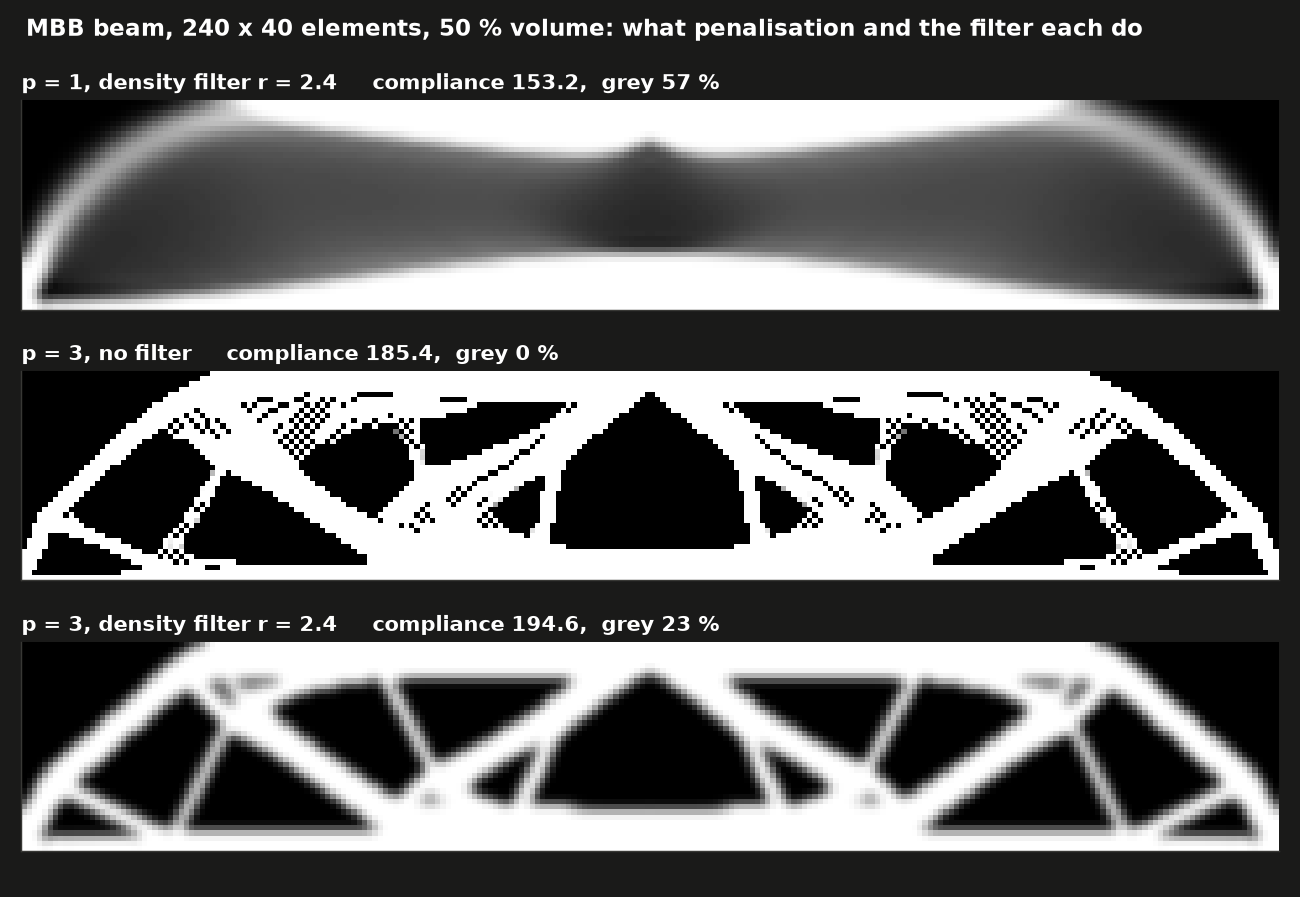
| Run (120 × 40 half beam, mirrored for display) | compliance | grey | checkerboard index |
|---|---|---|---|
| $p = 1$, filter $r_{\min} = 2.4$ | 153.2 | 57 % | – |
| $p = 3$, no filter | 185.4 | 0.2 % | 0.099 |
| $p = 3$, filter $r_{\min} = 2.4$ | 194.6 | 23 % | 0.014 |
The ranking of compliances is the lesson. The "best" number belongs to the unphysical grey design and the second best to the checkerboard. Both beat the clean truss only by exploiting modelling artefacts. The checkerboard index is the mean mixed second difference $|\rho_{i,j} - \rho_{i+1,j} - \rho_{i,j+1} + \rho_{i+1,j+1}|/2$, which is 1 for a perfect checkerboard and 0 for smooth fields.
Solvers: sparse LU vs Jacobi-CG vs AMG-CG
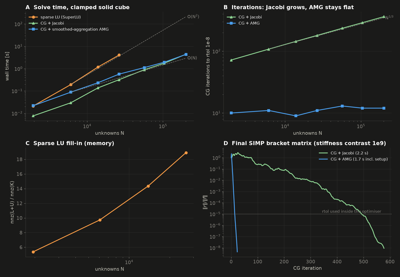
Clamped solid $n^3$ cube, tip shear, relative residual $10^{-8}$, wall-clock on a shared 8-core machine:
| $n$ | unknowns | sparse LU | LU fill nnz(L+U)/nnz(K) | Jacobi-CG its / time | AMG-CG its / time (setup) |
|---|---|---|---|---|---|
| 8 | 1,944 | 0.02 s | 5.4 | 72 / 0.008 s | 10 / 0.02 s (0.01) |
| 12 | 6,084 | 0.19 s | 9.7 | 108 / 0.03 s | 11 / 0.09 s (0.04) |
| 16 | 13,872 | 1.17 s | 14.4 | 144 / 0.14 s | 9 / 0.23 s (0.12) |
| 20 | 26,460 | 4.07 s | 18.9 | 180 / 0.32 s | 11 / 0.57 s (0.26) |
| 26 | 56,862 | – | – | 235 / 0.89 s | 13 / 1.11 s (0.50) |
| 32 | 104,544 | – | – | 289 / 1.75 s | 12 / 1.94 s (0.91) |
| 40 | 201,720 | – | – | 362 / 4.43 s | 12 / 4.35 s (2.29) |
- LU time grows as about $N^{2}$ between 6k and 26k unknowns, and its fill ratio keeps climbing. Extrapolated, 10⁶ unknowns would take about 1.5 hours. The benchmark stops LU at $n = 20$.
- Jacobi-CG iterations grow as $N^{0.35}$ (theory: $N^{1/3}$). AMG-CG stays at 9–13 iterations for a 100× range of $N$. AMG solutions agree with LU to 2×10⁻¹⁰.
- Honest result: at these sizes, on a homogeneous cube, the two CG variants cost about the same. Each AMG iteration costs about 14× a Jacobi iteration, and the setup is not free. The lines cross at about 2×10⁵ unknowns. Extrapolating the $N^{1/3}$ trend, Jacobi would need nearly 3,000 iterations per solve at 10⁸ unknowns (the scale of Aage et al. 2017), while multigrid stays near a dozen.
- Panel D shows the matrix the optimiser actually solves: the final bracket design with a 10⁹ stiffness contrast between solid and void. AMG-CG reaches 10⁻⁸ in 23 iterations (1.7 s including setup). Jacobi-CG needs 577 iterations (2.2 s) and spends its first 80 or so iterations going nowhere. Reading off the plot, it reaches the optimiser's 10⁻⁵ only after about 490 iterations, against about 12 for AMG.
Two things tried during development, and why they are not in the code:
- A full model without symmetry needed 62–65 AMG-CG iterations per load case at the start instead of 27, and its first design iteration took 26 s, against 6.5–10 s for the half model.
- Reusing the AMG hierarchy from the previous design iteration to save the setup was a disaster. After the first OC step the stiffnesses change by up to 40×, the stale preconditioner stopped being useful, and CG hit its 400-iteration cap on all four load cases (138 s for one design iteration, on a 2.67 mm grid).
Verification: cantilever vs beam theory
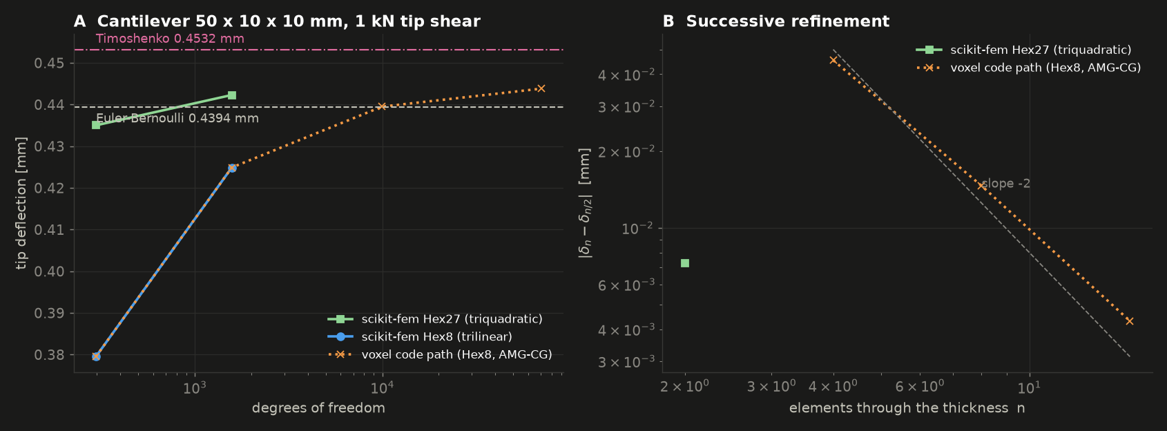
| Model | elements through thickness | dofs | tip deflection | vs Timoshenko | vs Euler–Bernoulli |
|---|---|---|---|---|---|
| scikit-fem Hex27 (triquadratic) | 1 | 297 | 0.4350 mm | −4.0 % | −1.0 % |
| scikit-fem Hex27 | 2 | 1,575 | 0.4423 mm | −2.4 % | +0.7 % |
| scikit-fem Hex8 (trilinear) | 2 | 297 | 0.3795 mm | −16.3 % | −13.6 % |
| scikit-fem Hex8 | 4 | 1,575 | 0.4249 mm | −6.2 % | −3.3 % |
| voxel code path (Hex8, Numba + AMG-CG) | 2 / 4 | 297 / 1,575 | identical to scikit-fem (2×10⁻¹³) | ||
| voxel code path | 8 | 9,963 | 0.4395 mm | −3.0 % | +0.0 % |
| voxel code path | 16 | 70,227 | 0.4438 mm | −2.1 % | +1.0 % |
- Asserted and passed: the fast path equals scikit-fem to 10⁻⁶ (actual 2×10⁻¹³). The finest Hex8 and Hex27 are within 3 % of both beam theories. Hex8 converges monotonically from below with observed order 1.64 → 1.76, heading for 2.
- Where the 3D answer sits. Richardson extrapolation of Hex8 ($n$ = 8, 16) gives 0.4453–0.4456 mm. A one-off Hex27 run at $n = 4$ (not in the default run: 115 s of scikit-fem assembly) gave 0.4445 mm. So the converged 3D solution is about 0.445 mm, +1.2–1.4 % above Euler–Bernoulli and −1.7–1.9 % below Timoshenko. The Timoshenko gap is model-form, not mesh. The FE clamp fixes the whole end face, so it stops that cross-section from warping and from Poisson contraction, while Timoshenko's shear coefficient assumes a section free to warp. The two beam theories bracket the 3D answer. (At $L/b = 10$ the two theories themselves differ by only 0.8 %, which is why this test uses a stubby beam.)
- Locking in one number: at the same 297 dofs, trilinear Hex8 is 15 % too stiff and triquadratic Hex27 is 2 % too stiff, both against the converged 0.445 mm. Topology optimisation tolerates Hex8 because the optimiser only needs relative stiffness between designs. An analyst certifying the final part would use quadratic tets or hexes.
All checks (default run)
[PASS] voxel/Numba/AMG path reproduces scikit-fem: max rel. diff 2.2e-13 (tol 1e-6)
[PASS] Hex8, n = 16 vs Timoshenko: 0.4438 mm vs 0.4532 mm (-2.07 %, tol 3 %)
[PASS] Hex8, n = 16 vs Euler-Bernoulli: 0.4438 mm vs 0.4394 mm (+1.01 %, tol 3 %)
[PASS] Hex27, n = 2 vs Timoshenko: 0.4423 mm vs 0.4532 mm (-2.41 %, tol 3 %)
[PASS] Hex27, n = 2 vs Euler-Bernoulli: 0.4423 mm vs 0.4394 mm (+0.67 %, tol 3 %)
[PASS] Hex8 converges monotonically from below: observed order [1.64 1.76] (-> 2 for trilinear hexes)
[PASS] AMG-CG agrees with sparse LU: max rel. diff 2.2e-10
[PASS] volume constraint met: 0.0800 vs 0.08
[PASS] compliance history converged: 0.23 % change over the last 10 iterations
[PASS] STL is watertight: 27184 triangles, no open edges
[PASS] density filter kills checkerboards: checkerboard index 0.099 unfiltered vs 0.014 filtered
[PASS] penalisation p = 3 removes grey: greyness 57 % (p=1) vs 0.2 % (p=3 raw) and 23 % (p=3 filtered: the filter's own blur band)
Run it
From the repo root:
uv run python L08_generative_bracket/sim.py
Runtime: 215 s (3.6 min) for the logged run below. An earlier identical run took 291 s while other jobs
had the CPU busy. The split is verification 9 s, solver benchmark 27 s, 2D MBB 9 s, bracket optimisation
151 s (45 iterations at 2.8–6.5 s each) plus 11 s of checks, and rendering 8 s. Threads are capped at 3 (OMP_NUM_THREADS,
NUMBA_NUM_THREADS), although nearly everything here is single-threaded C++ anyway (pyamg, SuperLU,
sparse mat-vecs). Everything is deterministic, so the numbers (not the timings) repeat exactly. To go faster or
finer, change H_VOX (voxel size, mm) and ITERS near the bottom of sim.py. A 2.67 mm grid (31,680
half-model voxels) looks smoother but takes about 1.5–2× longer.
It writes to output/:
| File | What |
|---|---|
hero.png |
the bracket with pin, bolts, design box and load arrows |
turntable.mp4 |
360° turntable, 1280×720, 4 s |
evolution.mp4 |
45 design iterations with the low-density cloud, compliance and volume |
von_mises.png |
von Mises envelope over the four load cases, two views |
bracket.stl |
the printable part (binary STL, mm, 27,184 triangles, watertight) |
convergence.png, history.csv |
per-iteration compliance (full part) per load case, volume, greyness, CG iterations, seconds |
verification.png |
cantilever tip deflection vs dofs, successive-refinement differences |
solver_benchmark.png |
LU vs Jacobi-CG vs AMG-CG, fill-in, residual histories on the SIMP matrix |
simp_filter_2d.png |
the MBB beam three ways |
Console output of the default run (abridged)
1/5 Verification: clamped 3D cantilever vs beam theory
                          model  n_thick  tip_mm  dofs  cg_its  vs_timoshenko_pct  vs_euler_bernoulli_pct
scikit-fem Hex27 (triquadratic)        1 0.43502   297       0           -4.01496                -0.98912
scikit-fem Hex27 (triquadratic)        2 0.44230  1575       0           -2.40845                 0.66803
    scikit-fem Hex8 (trilinear)        2 0.37952   297       0          -16.26042               -13.62061
    scikit-fem Hex8 (trilinear)        4 0.42490  1575       0           -6.24828                -3.29285
 voxel code path (Hex8, AMG-CG)        2 0.37952   297       1          -16.26042               -13.62061
 voxel code path (Hex8, AMG-CG)        4 0.42490  1575      14           -6.24828                -3.29285
 voxel code path (Hex8, AMG-CG)        8 0.43951  9963      16           -3.02520                 0.03183
 voxel code path (Hex8, AMG-CG)       16 0.44382 70227      19           -2.07360                 1.01343
2/5 Solver benchmark: sparse LU vs Jacobi-CG vs AMG-CG     (9 s)
  n =  8    1944 dofs  ... amg_its 10  jacobi_its 72   lu_s 0.0213  lu_fill 5.38
  n = 20   26460 dofs  ... amg_its 11  jacobi_its 180  lu_s 4.07    lu_fill 18.9
  n = 40  201720 dofs  ... amg_s 4.35  amg_its 12  jacobi_s 4.43  jacobi_its 362
3/5 SIMP and the density filter on the 2D MBB beam     (36 s)
4/5 Bracket topology optimisation     (45 s)
  half model: (55, 17, 20) voxels of 3.2 mm = 18700 elements; symmetric system 61932 dofs x 3 load cases + antisymmetric system 60756 dofs x 1
  bracket it   1  C = 2.1241e+06  vol = 0.0830  change = 0.162  cg its = [27, 28, 27, 27]  6.53 s
  bracket it  10  C = 7581.7  vol = 0.0800  change = 0.200  cg its = [11, 11, 11, 12]  3.41 s
  bracket it  45  C = 7095.8  vol = 0.0800  change = 0.058  cg its = [8, 7, 8, 8]  2.81 s      <- half model
  final SIMP matrix: AMG-CG 23 its / 1.7 s;  Jacobi-CG 577 its / 2.2 s, final residual 9.1e-09, error vs AMG 1.0e-06
  compliance: optimised 14192 N mm vs solid box 1694 N mm (x8.38 for 8 % of the material)
5/5 Rendering (PyVista) and STL     (207 s)
  STL: 27184 triangles, 79.2 cm^3 (6.5 % of the 1226 cm^3 box) = 351 g of Ti-6Al-4V
  von Mises envelope on the surface: 99th pct 192 MPa, max 221 MPa
Verification
  ... 12 x [PASS], see above
Total runtime 215 s
Code tour
Everything is in sim.py (about 800 lines, roughly a third of them rendering and plotting).
| Function | What it does |
|---|---|
voxel_fem(shape, h, E, nu) |
Structured 2D/3D voxel mesh (node ids via np.indices) and the element stiffness $\mathbf k_0$ from scikit-fem, integrated on one voxel and re-ordered from scikit-fem's global to local dof numbering |
set_supports(fe, fixed) |
A system = mesh + supports. Removes fixed dofs and precomputes the CSR pattern and the slot of each of the $24^2$ entries of every element (np.unique on row·N + col) |
scatter (Numba), assemble |
The assembly: data[slot] += E_e * k0. Then a CSR matrix is wrapped around the fixed pattern |
rigid_body_modes, amg, pcg, solve |
Near-null space, pyamg smoothed aggregation (sparse-LU coarse solve), CG with residual history, and multi-load-case solving with warm starts |
von_mises |
Element-centre strain from the trilinear shape-function gradients, then solid-material von Mises stress |
topopt(fe, cases, volfrac, rmin, ...) |
The optimiser. Cone filter as ndimage.correlate plus its adjoint, SIMP stiffness, solves for every (system, load-case) pair, self-adjoint sensitivities, OC with bisection on λ, history and snapshots. The same function runs the 2D MBB beams and the 3D bracket |
bracket(h) |
The GE-style problem: passive solids and voids from centroid geometry, clamped boss faces, symmetric and antisymmetric mid-plane conditions, pin-bore loads in N (lbf converted) |
beam_theory, cantilever_skfem, cantilever_voxel, verify_cantilever |
Verification: closed forms, scikit-fem end to end (Hex8/Hex27, FacetBasis traction, condense), and the same problem through the optimiser's code path |
solver_benchmark, design_matrix_check |
LU vs Jacobi-CG vs AMG-CG on cubes, and on the final SIMP matrix; solid-box compliance for scale |
mbb(penal, rmin), checkerboard |
The 2D ablation (p = 1, no filter, filter) and the checkerboard metric |
to_grid, part_surface |
Mirror the half model, pad, cell → point data, contour at 0.5, Taubin smooth, Loop subdivide, carry the stress field |
studio, look, hardware, envelope, load_arrows, render_bracket, write_mp4 |
PyVista scene (camera-attached key/fill/rim lights, SSAO), pin and bolts, design box, load arrows; hero, turntable, evolution, stress views, STL |
plot_*, verify, main |
Matplotlib figures, the 12 asserted checks, orchestration |
Simplifications & ceilings
- Voxels. The part is a staircase of 3.2 mm cubes. Smoothing makes it look organic but does not change the analysis, and surfaces, holes and fillets are only resolved to about one voxel. Body-fitted tets or adaptive octrees are the upgrade.
- Trilinear, fully integrated hexes lock in bending (see verification). That is fine for comparing designs inside the optimiser, but not for final stress numbers.
- Stress is a post-processing number. The optimisation minimises compliance only. There is no stress, fatigue or buckling constraint, and the reported stress (solid-material, element-centre, density-weighted onto the surface) ignores the stress concentrations that real fillets, bolt holes and pin contact would create. A real sign-off re-meshes the smoothed part and re-analyses it.
- Loads and supports are idealised. The pin load is spread evenly over the bore nodes (no pin contact or bearing pressure distribution). The bolts are fully clamped boss bottoms (no preload, no contact with the engine casing). The torsion case is one reading of the challenge's "5,000 lbf·in at the pin". The geometry is inspired by the GE bracket, not a copy of its CAD interface.
- Symmetry is imposed. The half model can only produce mirror-symmetric parts. For these load cases that is where the optimum lies, but it is an assumption.
- The density filter leaves a grey band, and the 0.5 isosurface cuts through it, so the STL (6.5 %) is lighter than the optimised density field (8 %). Heaviside projection with continuation would give a crisp 0/1 design.
- OC and a fixed 45 iterations. OC handles exactly one constraint. The stopping rule is an iteration cap, justified by the flat compliance history rather than by a KKT residual.
- Local optimum. The problem is non-convex, and other starting points, filter radii or continuation schedules give different (similar-compliance) topologies.
- No manufacturing constraints. The part is printable in the sense of being watertight, but no overhang angle or minimum wall was enforced, so a real print would need supports or an AM filter.
- AMG rebuilt every iteration (about 0.5 s of each 3 s). Recycling the hierarchy with a trigger on CG iteration counts, or geometric multigrid on the voxel hierarchy, would be the next speed-up. Blind reuse was tried and failed (see Solvers).
Go further
- Crisp designs. Add a Heaviside projection $\bar\rho = \frac{\tanh(\beta\eta) + \tanh(\beta(\tilde\rho-\eta))}{\tanh(\beta\eta) + \tanh(\beta(1-\eta))}$ with $\beta$ doubled every 20 iterations (Wang, Lazarov & Sigmund 2011), and compare greyness, STL mass and compliance with this run.
- Stress-constrained design. Replace OC with MMA (Svanberg 1987, e.g. the
nloptormmapyimplementations), add a p-norm von Mises constraint with relaxed stresses (Le et al. 2010), and watch the lug crowns and leg roots thicken. - Print-ready. Add Langelaar's (2017) additive-manufacturing overhang filter for a chosen build direction, then
slice
bracket.stlin PrusaSlicer or Cura and compare support volume with and without it. - Scale up. Replace pyamg with a matrix-free geometric multigrid on the voxel hierarchy (Amir, Aage & Lazarov 2014), or run the same problem in PETSc TopOpt, and push to 10⁶–10⁷ voxels. Rerun the solver benchmark to find where Jacobi-CG finally loses in wall time.
- Rebuild it in an industry tool. Load the four load cases into Altair Inspire (free student edition) or Fusion 360 Generative Design with the same keep-in/keep-out regions and 8 % volume target, and compare topology, mass and compliance. Then import our STL into Ansys Mechanical or Abaqus, mesh it with quadratic tets (C3D10) and see how far the voxel-level stresses were from the body-fitted ones.
References
- M. P. Bendsøe & O. Sigmund, Topology Optimization: Theory, Methods and Applications, Springer (2003).
- M. P. Bendsøe, "Optimal shape design as a material distribution problem", Structural Optimization 1, 193 (1989).
- M. P. Bendsøe & N. Kikuchi, "Generating optimal topologies in structural design using a homogenization method", Comput. Methods Appl. Mech. Eng. 71, 197 (1988).
- O. Sigmund, "A 99 line topology optimization code written in Matlab", Struct. Multidisc. Optim. 21, 120 (2001).
- E. Andreassen, A. Clausen, M. Schevenels, B. S. Lazarov & O. Sigmund, "Efficient topology optimization in MATLAB using 88 lines of code", Struct. Multidisc. Optim. 43, 1 (2011).
- K. Liu & A. Tovar, "An efficient 3D topology optimization code written in Matlab", Struct. Multidisc. Optim. 50, 1175 (2014).
- T. E. Bruns & D. A. Tortorelli, "Topology optimization of non-linear elastic structures and compliant mechanisms", Comput. Methods Appl. Mech. Eng. 190, 3443 (2001).
- B. Bourdin, "Filters in topology optimization", Int. J. Numer. Methods Eng. 50, 2143 (2001).
- A. R. Díaz & O. Sigmund, "Checkerboard patterns in layout optimization", Structural Optimization 10, 40 (1995).
- O. Sigmund & J. Petersson, "Numerical instabilities in topology optimization: a survey on procedures dealing with checkerboards, mesh-dependencies and local minima", Structural Optimization 16, 68 (1998).
- F. Wang, B. S. Lazarov & O. Sigmund, "On projection methods, convergence and robust formulations in topology optimization", Struct. Multidisc. Optim. 43, 767 (2011).
- K. Svanberg, "The method of moving asymptotes — a new method for structural optimization", Int. J. Numer. Methods Eng. 24, 359 (1987).
- C. Le, J. Norato, T. Bruns, C. Ha & D. Tortorelli, "Stress-based topology optimization for continua", Struct. Multidisc. Optim. 41, 605 (2010).
- M. Langelaar, "An additive manufacturing filter for topology optimization of print-ready designs", Struct. Multidisc. Optim. 55, 871 (2017).
- N. Aage, E. Andreassen, B. S. Lazarov & O. Sigmund, "Giga-voxel computational morphogenesis for structural design", Nature 550, 84 (2017).
- O. Amir, N. Aage & B. S. Lazarov, "On multigrid-CG for efficient topology optimization", Struct. Multidisc. Optim. 49, 815 (2014).
- P. Vaněk, J. Mandel & M. Brezina, "Algebraic multigrid by smoothed aggregation for second and fourth order elliptic problems", Computing 56, 179 (1996).
- A. George, "Nested dissection of a regular finite element mesh", SIAM J. Numer. Anal. 10, 345 (1973).
- A. G. M. Michell, "The limits of economy of material in frame-structures", Phil. Mag. 8, 589 (1904).
- G. R. Cowper, "The shear coefficient in Timoshenko's beam theory", J. Appl. Mech. 33, 335 (1966).
- T. J. R. Hughes, The Finite Element Method: Linear Static and Dynamic Finite Element Analysis, Dover (2000).
- G. Taubin, "A signal processing approach to fair surface design", Proc. SIGGRAPH '95, 351 (1995).
- W. E. Lorensen & H. E. Cline, "Marching cubes: a high resolution 3D surface construction algorithm", Proc. SIGGRAPH '87, 163 (1987).
- T. Gustafsson & G. D. McBain, "scikit-fem: a Python package for finite element assembly", J. Open Source Softw. 5, 2369 (2020).
- N. Bell, L. N. Olson & J. Schroder, "PyAMG: algebraic multigrid solvers in Python", J. Open Source Softw. 7, 4142 (2022).
- C. B. Sullivan & A. A. Kaszynski, "PyVista: 3D plotting and mesh analysis through a streamlined interface for the Visualization Toolkit (VTK)", J. Open Source Softw. 4, 1450 (2019).
- GrabCAD, GE jet engine bracket challenge (2013). The load cases and Ti-6Al-4V material used here follow the challenge brief.